SHAPE RETRIEVAL USING CONTOUR FEATURES AND
DISTANCE OPTIMIZATION
Daniel Carlos Guimar
˜
aes Pedronette and Ricardo da S. Torres
Institute of Computing, University of Campinas (Unicamp), Campinas, Brazil
Keywords:
Shape Description, Content-based image retrieval, Distance optimization.
Abstract:
This paper presents a shape descriptor based on a set of features computed for each point of an object contour.
We also present an algorithm for distance optimization based on the similarity among ranked lists. Experi-
ments were conducted on two well-known data sets: MPEG-7 and Kimia. Experimental results demonstrate
that the combination of the two methods is very effective and yields better results than recently proposed shape
descriptors.
1 INTRODUCTION
The huge growth of image collections and multime-
dia resources available and accessible through various
technologies is not new for years. The same can be
said of the research motivated by the need of meth-
ods for indexing and retrieval these data. For two
decades, several models of Content-Based Image Re-
trieval - CBIR have been proposed using features such
as shape, color, and texture for retrieving images.
Shape is clearly an important cue for recogni-
tion since humans can often recognize characteris-
tics of objects solely on the basis of their shapes.
This distinguishes shape from other elementary vi-
sual features, which usually do not reveal object iden-
tity (Adamek and OConnor, 2004). Several shape
descriptors proposed in the literature analyze certain
features of shapes, measuring properties associated
with each pixel of the object contour, such as an-
gle (Arica and Vural, 2003) and area of regions (Ala-
jlan et al., 2007). Those works have shown that many
of those features are able to characterize the shape
complexity of objects. However, most approaches
uses only one feature.
In this paper, we propose a new shape description
model that allows the combination of several features
computed for each pixel of an object contour. We
also propose a new distance optimization method for
improving the effectiveness of CBIR systems. This
method exploits the similarity among ranked lists to
redefine the distance among images.
Several experiments were conducted on two
widely used image collections: MPEG-7 and Kimia.
Experiment results demonstrate that the combination
of the proposed methods yields effectiveness perfor-
mance that are superior than several shape descriptors
recently proposed in the literature.
2 BASIC CONCEPTS
Several feature functions proposed in this paper com-
pute feature values for each point of the object con-
tour by analyzing neighbour pixels. The concept of
neighborhood is also used to classify features as lo-
cal, regional, or global. Two pixels are considered
neighbors if their distance is not greater than a radius
of analysis, which is defined below.
Definition 1. The radius of analysis r
a
=
max(D
center
) × χ, where D
center
={ d
c
0
,d
c
1
, ..., d
c
n
}
is a set in domain R, and each element d
c
i
is defined
by the Euclidean distance of each contour pixel to the
center of mass of the object, and χ is a constant.
Definition 2. A contour feature f
j
can be defined as
set of real values f
j
={ f
0 j
, f
i j
, . . . , f
n j
} (one for each
contour pixel p
i
) that represents features that can be
extracted by a feature function F
j
: p
i
→ f
i j
, where j
identifies the feature, i defines the pixel p
i
of the object
contour and f
i j
∈ R is the value of feature f
j
for the
pixel p
i
.
197
Carlos Guimarães Pedronette D. and da S. Torres R. (2010).
SHAPE RETRIEVAL USING CONTOUR FEATURES AND DISTANCE OPTIMIZATION.
In Proceedings of the International Conference on Computer Vision Theory and Applications, pages 197-202
DOI: 10.5220/0002837201970202
Copyright
c
 SciTePress

3 SHAPE DESCRIPTION BASED
ON CONTOUR FEATURES
The proposed descriptor is based on the combina-
tion of features that describe the contour of an object
within an image. These features can be classified as
local, regional, or global, according to the proximity
of the pixels that are analyzed.
3.1 Feature Vector Extraction
Let S
F
={F
0
, F
1
, . . . , F
m
} be a set of feature functions
based on contour, S
f
={ f
0
, f
1
, . . . , f
m
} be a set of
features based on contour, and C
D
I
= {p
0
, p
1
,..., p
n
}
be a set of pixels that defines the contour of an ob-
ject. The feature vector v
b
I
= (v
1
, v
2
, . . . , v
d
) has d =
n × m dimensions and can be represented by a matrix
f
v
, where each cell is given by the value of feature F
j
applied to the pixel p
i
, i.e., f
v
[i, j]=F
j
(p
i
). The fea-
ture vector extraction can be performed by applying a
feature function F
j
to each contour pixel p
i
.
3.2 Local Features
Local features aims to characterize relevant properties
in a small neighborhood of a contour pixel p
i
. The ex-
traction of local features is based on analyzing pixels
wich are within the area defined by the radius of anal-
ysis (see Definition 1) from the pixel p
i
. Changes in
other regions of the object does not influence the val-
ues of local features.
Normal Angle. The normal angle Θ
n
is defined as the
angle between the normal vector and the horizontal
line.
Concavity. this feature aims to characterize the con-
cavity/convexity around the current pixel p
i
. Pixels
in concave regions present high values, whereas pix-
els in convex regions present low values. The con-
cavity is computed from radially sample lines, which
are traced emerging from the current pixel p
i
. Sample
lines are traced starting from normal vector Θ
n
to both
side of this vector, with a angular increment of c
◦
a
or
−c
◦
a
until increments reachs Θ
n
+ 180
◦
or Θ
n
− 180
◦
.
For each line, it is verified if object pixels are found
by applying function f
inOb ject
. This function is de-
fined as follows: let p
j
be a pixel at a distance r
a
from the pixel p
i
at the direction of the angle Θ
j
, and
let S
line
= {p
k
0
, p
k
1
,..., p
k
n
} be the sample line (set of
points) traced from p
j
at Θ
j
direction. Let O
D
I
be
the set of pixels that composes the analyzed object.
Function f
inOb ject
is defined as follow:
f
inOb ject
(p
i
,Θ
j
) =



2, if p
j
∈ O
D
I
1, if p
j
/∈ O
D
I
, and ∃p
k
l
∈ O
D
I
0, otherwise
The value of concavity is the number of sample
lines that are traced after function f
inOb ject
assumes
value 2. Algorithm 1 shows how to compute the con-
cavity feature f
concavity
[p
i
] of a pixel p
i
. Variable f lag
is used to determine if pixel p
j
∈ O
D
I
was found.
Opposite Opening. This feature aims to identify
contour segments that are associated with branches
or stems of the object, such as legs of animals and
tree branches. Only pixels of these segments have
the value of the opposite opening different of zero.
The method to compute opposite opening is similar
to that used for computing concavity. When tracing
the sample lines starting from the normal vector di-
rection, pixels belonging to the object are found at a
distance r
a
( f lag = 1). After further angular varia-
tions, sample lines do not intercept object pixels at a
distance r
a
. Only these sample lines are used for com-
puting the value of the opposite opening. Algorithm 1
shows the main steps used to compute this feature.
3.3 Global Features
We can obtain some features analyzing global proper-
ties of objects. These features are classified as global
fetaures due to the fact that changes in any region of
the object affect their values.
Distance to Center of Mass. The distance to center
of mass d
c
i
is given by the Euclidean distance between
current pixel p
i
and the pixel that represents the center
of mass p
c
.
Angle to Center of Mass. Let ~v
ac
be a vector with
origin at current pixel p
i
in direction to the pixel of
the center of mass p
c
, the angle to center of mass Θ
c
is given by the angle between this vector and the hor-
izontal line.
3.4 Regional Features
Regional features characterize shape properties that
depend on both global features (such center of mass)
and the local features (such as normal angle).
Opposite Distance. The opposite distance d
o
is com-
puted from a sample line, which is traced emerging
from the current pixel p
i
in opposite direction to the
normal vector. Let p
f
be the contour pixel defined by
the first intersection of this sample line and the object
contour. The opposite distance is obtained by com-
puting the Euclidean distance between the pixel p
i
and the pixel p
f
. The opposite distance is normalized
by the maximum distance value
VISAPP 2010 - International Conference on Computer Vision Theory and Applications
198

Difference between Normal Angle and Angle to the
Center of Mass. This feature is computed from abso-
lute distante between values of normal angle Θ
n
and
the angle to the center of mass Θ
c
.
Opening. This feature aims to characterize informa-
tion about the extent of the branches in a neighbor-
hood of current pixel p
i
. Similarly to the computation
of the concavity, radially sample lines are traced and,
for each angular increment, a test is performed. The
value of opening f
opening
is equal to the value of con-
cavity f
concavity
(where a pixel belonging to the object
is located from a distance r
a
of the pixel p
i
) plus the
number of sample lines that intercept the object for a
distance greater than r
a
. Algorithm 1 presents steps
to perform the computation of this feature.
Algorithm 1. Computation of Concavity, Opening, and Op-
posite Opening.
Require: Current pixel p
i
Ensure: Computed features for p
i
: concavity, opening,
and opposite opening
1: f
concavity
[p
i
] ← 0
2: f
opening
[p
i
] ← 0
3: f
oppositeOpening
[p
i
] ← 0
4: f lag ← 0
5: for Θ
j
= Θ
n
to (Θ
n
+ / − 180
◦
) do
6: if f
inOb ject
(p
i
,Θ
j
) = 2 then
7: f lag ← 1
8: end if
9: f
concavity
[p
i
] ← f
concavity
[p
i
] + f lag
10: if f lag or f
inOb ject
(p
i
,Θ
j
) = 1 then
11: f
opening
[p
i
] ← f
opening
[p
i
] + 1
12: end if
13: if f lag and f
inOb ject
(p
i
,Θ
j
) 6= 2 then
14: f
oppositeOpening
[p
i
] ← f
oppositeOpening
[p
i
] + 1
15: end if
16: Θ
j
← Θ
j
+ / − c
a
17: end for
In addition to the feature vectors, three other mea-
sures are computed for a given object: area, perimeter,
and the maximum distance from the center of mass.
The feature vectors are sampled to the same size
for all images in the collection. We used feature vec-
tors with 1000 elements.
3.5 Histogram-based Features
A great challenge for matching feature vectors re-
lies on the fact that many objects, though with sim-
ilar shapes, present different sizes of contour for cor-
responding segments. One solution to alleviate this
problem consists in using histogram-based features
for characterizing the shape complexity. Histograms
are computed as follows: considering the interval
[0, f
max
], where f
max
represents the maximum value
of a particular feature, we divide this interval in h
sub-intervals (in our experiments, h = 11). For each
sub-interval, we compute the number of contour pix-
els whose feature value belongs to the sub-interval
range. Thus, using the feature vector f
v
as input, we
can compute a histogram for each feature f
j
of each
object. Only for Normal Angle and Angle to Center
of Mass, which are sensitive to rotation, histograms
are not computed.
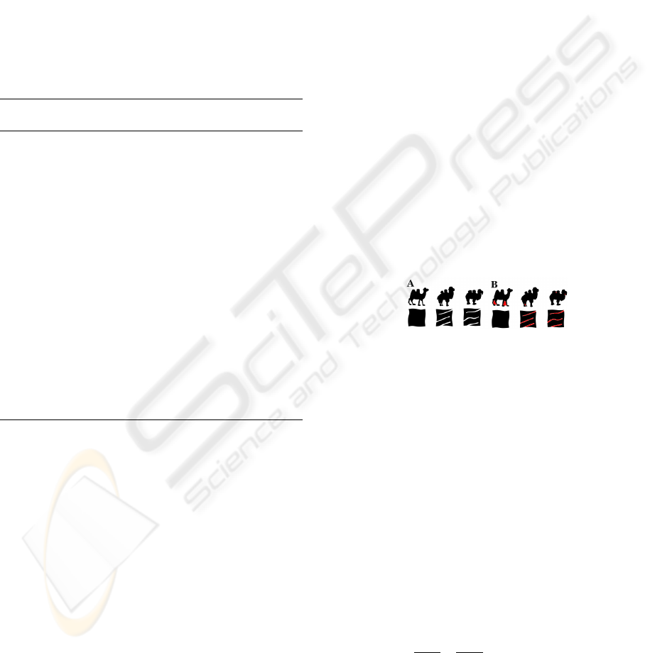
3.6 Irrelevant Contour Segments
There are segments of contour which have some in-
stability in the shape contour. Due to small changes
in the angle/perspective that the image is seen, such
segments may disappear in the visual perception of
the contour of the object. Figure 1 shows examples of
objects (part A), and the irrelevant segments of con-
tour in red (part B).
These segments can be detected by computing a
moving average of the opening feature for the pixels
of the contour. When the value of the moving average
of the opening is too high (greater than a threshold
th
opening
), these points are discarded for the purpose
of matching and distance computation. The size s
m
of
the moving average used for the experiments was s
m
= 10 and threshold th
opening
= 45.0.
Figure 1: Irrelevant segments of contour.
4 DISTANCE COMPUTATION
4.1 Matching for Rotation Invariance
Feature vectors of similar objects may differ due to ro-
tations. In order to solve this problem, a matching is
performed. One feature vector is taken as reference,
and the second feature vector is shifted considering
different offset values. For each shift, the distance be-
tween the two feature vectors is computed. We call
of ideal offset o
m
for the matching that produces the
minimun value for the computed distance.
The features used for similarity distance compu-
tation during the matching are the distance to the
center of mass and opposite distance. The simi-
larity distance for matching is defined as follows:
dist
matching
= dist
c
+ dist
o
, where dist
c
and dist
o
de-
fine the value of distance for features distance to the
center of mass and opposite distance, respectively.
They are computed by applying the L1 distance.
SHAPE RETRIEVAL USING CONTOUR FEATURES AND DISTANCE OPTIMIZATION
199

4.2 Feature and Histogram Distances
The L1 distance is used after applying the best off-
set for computing the distance for a feature f
j
be-
tween two objects. Distances are normalized as fol-
lows: dist
f
j
= (avg( f
j
)/max( f
j
)
2
) × dist
f
j
, where f
j
defines the values of feature j for each pixel p
i
of
the contour, avg( f
j
) defines the average of f
j
, and
max( f
j
) defines the maximum value of f
j
, consider-
ing all images in the collection.
The L1 distace is also used to compute the dis-
tance between two histograms.
4.3 Final Distance
The final distance dist
f inal
is computed as follow:
dist
f inal
= (dist
aa
× w
aa
) + (dist
ca
× w
ca
) + (dist
gr
×
w
gr
) + (dist
h
× w
h
), where: dist
aa
is the sum of dis-
tances for angle to center of mass and normal angle;
dist
ca
is the sum of distances for concavity, opening
and opposite opening; dist
gr
is the sum of distances
for the opposite distance, distance of center of mass,
and distance between normal angle and angle to the
center of mass; dist
h
is the sum of histogram dis-
tances.
The final distance depends also on the similarity
of overall measures of the objects, such as area and
perimeter. We propose to adjust the value of the final
distance given these similarity values. Our strategy
works as follows: the values of area and perimeter
are normalized using the maximum distance of cen-
ter of mass (for scale invariation). For each normal-
ized values (area and perimeter), we check if the dif-
fence of the area (perimeter) values is greater than
a threshold th
area
(th
perimeter
). If so, the value of
the final distance receives a penality p > 1, that is
dist
f inal
← dist
f inal
× p. We used w
aa
= 12, w
ca
= 3,
w
gr
= 60, w
h
= 1, th
area
= 0.7, th
perimeter
= 3.5, and
p = 1.1.
5 DISTANCE OPTIMIZATION
ALGORITHM
We can use the features defined in previous sections
to process shape-based queries in an image collection
C = {img
1
,img
2
,...,img
n
}. For a given query image
img
q
, we can compute the distance among img
q
and
all images of collection C. Next, collection images
can be ranked according to their similarity to img
q
,
generating a ranked list R
q
. We expect that similar im-
ages to img
q
are placed at first positions of the ranked
list R
q
. In fact, it is possible to use the proposed fea-
tures to compute the distances among all images of C.
Let the matrix W be a distance matrix, where W(k,l)
is equal to the distance between images img
k
∈ C and
img
l
∈ C. It is also possible to compute ranked lists
R
img
k
for all images img
k
∈ C.
5.1 The Algorithm
Our strategy for distance optimization relies on ex-
ploiting the fact that if two images are similar, their
ranked lists should be similar as well. Basically, we
propose to redefine the distance among images, given
the similarity of their ranked lists. A clustering ap-
proach is used for that. Images are assigned to the
same cluster if they have similar ranked lists. Next,
distances among images belonging to same cluster are
updated (decreased). This process is repeated until
the “quality” of the formed groups does not improve
and, therefore, we have “good” ranked lists. We use
a cohesion measure for determining the quality of a
cluster.
Let C = {img
1
,img
2
,...,img
n
} be a set (or clus-
ter) of images. Let R
img
k
be the ranked list of query
image img
k
∈ C with size images. R
img
k
is created us-
ing the distances among images. The cohesion of C is
computed based on its first top
n
results of the ranked
lists R
img
k
. It is defined as follows:
cohesion(C) =
∑
size
j=0
∑
top
n
i=0
(top
n
−i)×(top
n
/c)×S(i)
size
2
,
where c is a constant
1
that defines a weight for a posi-
tion in the ranked list and S is a function S: i → {0,1},
that assumes value 1, if C contains the image ranked
at position i of the ranked list defined by query image
img
j
∈ C or assumes value 0, otherwise. Algorithm 2
presents the proposed distance optimization method
used to redefine distances among images.
Algorithm 2 . Distance Optimization Algorithm.
Require: Distance matrix W
Ensure: Optimized distance matrix W
o
1: lastCohesion ← 0
2: currentCohesion ← computeCohesion(W )
3: while curCohesion > lastCohesion do
4: Cls ← createClusters(W )
5: W ← updateDistances(W,Cls)
6: lastCohesion ← currentCohesion
7: currentCohesion ← computeCohesion(W )
8: end while
9: W
o
← W
Function computeCohesion(W ) returns the av-
erage cohesion considering all clusters defined by
ranked lists. Function createClusters() is responsi-
ble for creating clusters. It is detailed in Section 5.2.
Finally, function updateDistances() verifies, for each
pair of images, if they are in the same group. If so, the
1
We use c=10 in our experiments.
VISAPP 2010 - International Conference on Computer Vision Theory and Applications
200

distance between them is updated, i.e., multiplied by
a constant c
mult
< 1. In our experiments, c
mult
= 0.95.
5.2 Clustering Algorithm
We use a graph-based approach for clustering. Let
G(V,E) be a directed and weighted graph, where a
vertex v ∈ V represents an image. The weight w
e
of
edge e = (v
i
,v
j
) ∈ E is defined by the ranking position
of image img
j
(v
j
) at the ranked list of img
i
(v
i
).
Definition 3. Let (k,l) be a ordered pair. Two im-
ages img
i
and img
j
are (k,l)-similar, if w
e
i, j
≤ k and
w
e
j,i
≤ l, where e
i, j
= (img
i
,img
j
) is the edge between
images img
i
and img
j
.
Definition 4. Let S
p
= {(k
0
,l
0
),(k
1
,l
1
), . . . , (k
m
,l
m
)}
be a set of ordered pairs. Two images, img
i
and img
j
,
are cluster-similar according to S
p
, if ∃(k
a
,l
a
) ∈
S
p
|img
i
and img
j
are (k
a
,l
a
)-similar.
Figure 2 illustrates how to determine if two im-
ages are cluster-similar. In this example, S
p
=
{(1,8),(2,6),(3,5),(4,4)}. First, it is checked if
img
1
and img
2
are (1,8)-similar. In this case, if the
image ranked at the first position of ranked list R
img
1
is at one of the eight first positions of ranked list R
img
2
,
images img
1
and img
2
are (1,8)-similar. If not, the
second pair of S
p
is used, and so on.
Figure 2: Example of cluster-similarity be-
tween images img
1
and img
2
with regard to
S
p
= {(1,8), (2,6),(3, 5),(4,4)}.
Algorithm 3 shows the main steps for clustering
images. The main step of the algorithm is the func-
tion evaluateSimilarity. This function is in charge of
creating an initial set of clusters. Algorithms 4 and 5
show the main steps for creating image clusters. As
it can be observed in step 7 of Algorithm 5, two im-
ages are assigned to the same cluster only if they are
cluster-similar (Definition 4), according to a set S
p
.
Function mergeClusters(Clusters) deals with
clusters with only one image. Let R
img
be the ranked
list of the image of such a cluster. If the cohesion
of the top
nToAdd
images in R
img
are greater than a
threshold (th
cohesion
), then img is added to the cluster
that has more images of R
img
. This function is also
in charge of merging small-size clusters. A small-
size cluster is added to a larger cluster. If the co-
hesion of this new group is greater than a threshold
th
cohesion
, these clusters are merged. Furthermore, the
new group should have a cohesion greater than the
average cohesion of the initial clusters. Weights are
defined by the size of the initial clusters.
Algorithm 3. Clustering Algorithm.
Require: Graph G, S
1
= {(1,8),(2, 6),(3,5), (4,4)}, S
2
=
{(1,6), (2,4),(3, 3)}.
Ensure: A set of clusters Cls.
1: Cls ← null
2: Cls ← evaluateSimilarity(G(V,E), S
1
,Cls)
3: Cls ← mergeClusters(Cls)
4: Cls ← divideClusters(Cls)
5: Cls ← evaluateSimilarity(G(V,E), S
2
,Cls)
6: Cls ← mergeClusters(Cls)
Algorithm 4. Algorithm evaluateSimilarity.
Require: Graph G = (V,E) and S
p
.
Ensure: Set of clusters Cls.
1: Cls = { }
2: for all i such that 0 ≤ i ≤
|
V
|
do
3: currentCluster = { }
4: processImage (img
i
,G,S
p
)
5: Cls ← Cls ∪ currentCluster
6: end for
Algorithm 5. Algorithm processImage.
Require: Image img
i
, Graph G = (V, E), and S
p
.
1: if alreadyProcessed(img
i
) then
2: return
3: end if
4: currentCluster = currentCluster ∪ img
i
5: for all j such that 0 ≤ j ≤
|
top
n
|
do
6: img
j
← w
e
i, j
7: if clusterSimilar(img
i
,img
j
,S
p
) then
8: if not alreadyProcessd(img
j
) then
9: processImage(img
j
,G,S
p
)
10: else
11: currentCluster ← currentCluster ∪
clusterOf(img
j
)
12: end if
13: end if
14: end for
If the cohesion of a formed cluster is less than
threshold th
cohesion
, this cluster is splited and the sta-
tus of its images is set to “non-processed” in the
divideClusters(Clusters) function. These images are
processed in steps 5 and 6 of Algorithm 3. In this
case, S
2
= {(1, 6), (2, 4), (3, 3)} is used to defined the
similarity among images.
SHAPE RETRIEVAL USING CONTOUR FEATURES AND DISTANCE OPTIMIZATION
201

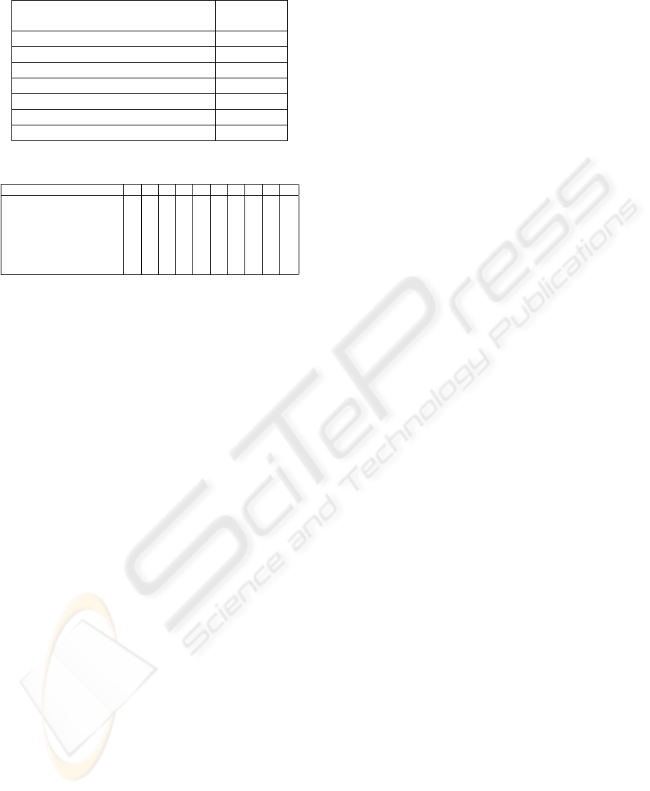
Table 1: Results comparison in MPEG-7 dataset.
Descriptors Retrieval
Rate
BAS (Arica and Vural, 2003) 82.37%
CFD 84.43%
DSW (Alajlan et al., 2007) 85.03%
IDSC+DP (Ling and Jacobs, 2007) 85.40%
DSW+Global (Alajlan et al., 2007) 87.23%
Graph Trans. (Yang et al., 2008) 91.00%
CFD+DistOpt 92.56%
Table 2: Results of experiments in Kimia dataset.
Descriptors 1
o
2
o
3
o
4
o
5
o
6
o
7
o
8
o
9
o
10
o
SC (Sebastian et al., 2004) 97 91 88 85 84 77 75 66 56 37
CFD 99 98 98 99 97 90 86 86 68 56
IDSC+DP 99 99 99 98 98 97 97 98 94 79
Shape Tree (Felzenszwalb
and Schwartz, 2007)
99 99 99 99 99 99 99 97 93 86
CFD + DistOpt 98 99 99 99 98 99 99 97 98 99
Graph Trans. 99 99 99 99 99 99 99 99 97 99
6 EXPERIMENTAL RESULTS
We conducted experiments in two image databases,
both widely used in the literature.
The MPEG-7 data set consists of 1400 silhouette im-
ages grouped into 70 classes. Each class has 20 dif-
ferent shapes. The retrieval rate is measured by the
number of shapes from the same class among the
40 most similar shapes. The following values were
defined for the parameters used in the distance op-
timization method: top
n
= 40, th
cohesion
= 70, and
top
nToAdd
= 10. Table 1 shows the results of sev-
eral descriptors using the MPEG-7 data set. The pro-
posed methods are named CFD and CFP + DistOpt.
CFP + DistOpt considers both the feature descrip-
tion approach and the proposed distance optimiza-
tion method. As it can be observed, CFP + DistOpt
has the best effectiveness performace when compared
with several well-known shape descriptors.
We also present experimental results on the Kimia
Data Set. This data set contains 99 shapes grouped
into nine classes. In this case, the following param-
eters’ values used in the distance optimization were
used: top
n
= 15, th
cohesion
= 7, and top
nToAdd
= 4.
The retrieval results are summarized as the number of
shapes from the same class among the first top 1 to
10 shapes (the best possible result for each of them
is 99). Table 2 lists the number of correct matches of
several methods. Again we observe that our approach
yields a very high retrieval rate, being superior to sev-
eral well-know shape descriptor.
7 CONCLUSIONS
In this paper, we have presented a shape description
approach that combines features extracted from ob-
ject contour. This paper has also presented a new op-
timization approach for reranking results in image re-
trieval systems. Several experiments were conducted
using well-known data sets. Results demonstrate that
the combination of both methods yield very high ef-
fectiveness performance when compared with impor-
tant descriptors recently proposed in the literature.
Future work includes the investigation of new fea-
tures to be incorporated into the proposed description
framework. We also plan to use the distance optimiza-
tion method with color and texture descriptors.
ACKNOWLEDGEMENTS
Authors thank CAPES, FAPESP and CNPq for finan-
cial support.
REFERENCES
Adamek, T. and OConnor, N. E. (2004). A multiscale
representation method for nonrigid shapes with a sin-
gle closed contour. IEEE Trans. Circuits Syst. Video
Techol., 14 i5:742–753.
Alajlan, N., El Rube, I., Kamel, M. S., and Freeman, G.
(2007). Shape retrieval using triangle-area represen-
tation and dynamic space warping. Pattern Recogn.,
40(7):1911–1920.
Arica, N. and Vural, F. T. Y. (2003). Bas: a perceptual shape
descriptor based on the beam angle statistics. Pattern
Recogn. Lett., 24(9-10):1627–1639.
Felzenszwalb, P. F. and Schwartz, J. D. (2007). Hierarchical
matching of deformable shapes. CVPR, pages 1–8.
Ling, H. and Jacobs, D. W. (2007). Shape classification
using the inner-distance. PAMI, 29(2):286–299.
Sebastian, T. B., Klein, P. N., and Kimia, B. B. (2004).
Recognition of shapes by editing their shock graphs.
PAMI, 26(5):550–571.
Yang, X., Bai, X., Latecki, L. J., and Tu, Z. (2008). Improv-
ing shape retrieval by learning graph transduction. In
ECCV, pages 788–801.
VISAPP 2010 - International Conference on Computer Vision Theory and Applications
202