CHANGE-POINT DETECTION ON THE LIE GROUP SE(3) FOR

SEGMENTING GESTURE-DEFINED SPATIAL RIGID MOTION

Loic Merckel and Toyoaki Nishida

Graduate School of Informatics, Kyoto University, Japan

Keywords:

Change-point detection, Lie group, Rigid body motion segmentation, Special Euclidean group, Exponential

map.

Abstract:

Common CAD interfaces for editing spatial motion of virtual objects, which includes both position and ori-

entation information, are often hampered by complexity and lack of intuitiveness. As the demand for motion

data is increasing, e.g., in computer graphics or mixed reality, the development of new interfaces that oﬀer a

natural means of specifying arbitrary motion becomes essential. A solution consists in relying on live motion

capture systems to record user’s gestures through space. In this context, we present a novel method for dis-

covering change-points in a time series of elements in the set of rigid-body motion in space SE(3). The goal is

to segment gesture-deﬁned motion with in mind the development of a method for enhancing the user’s intent.

Although numerous change-points detection techniques are available for dealing with scalar, or vector, time

series, the generalization of these techniques to more complex structures may require overcoming diﬃcult

challenges. The group SE(3) does not satisfy closure under linear combination. Consequently, most of the

statistical properties, such as the mean, cannot be properly estimated in a straightforward manner. We present

a method that takes advantage of the Lie group structure of SE(3) to adapt a diﬀerence of means method.

Especially, we show that the change-points in SE(3) can be discovered in its Lie algebra se(3) that forms a

vector space. The performance of our method is evaluated through both synthetic and real data.

1 INTRODUCTION

The growing progress in capturing motions, includ-

ing both position and orientation data, has motivated

some initiatives (e.g., (Merckel and Nishida, 2009)) to

develop new interfaces, for generating hand-deﬁned

motions, as an alternative to the conventional, and

overwhelming, WIMP-based interfaces (van Dam,

1997) of CAD software. An important application

is to provide a wide range of users with an eﬀective

means of creating animated 3D contents for Mixed

Reality (MR) environments. In this vein, (Merckel

and Nishida, 2009) present a hand-held MR interface,

which consists of a tablet PC equipped with a six-

degree-of-freedom (6-DOF) orientation and position

sensor, for animating 3D virtual items. To do so, the

user naturally describes the 6-DOF trajectory in space

by moving the hand-held system as if it was the item.

Such a technique suﬀer from a two-fold draw-

back. First, the motion capture process is, to some ex-

tent, limited in precision and may contain noise. Sec-

ond, user’s inputs are hampered by what (Sezgin and

Davis, 2004) refer to as “imperfect motor control”,

i.e., the user’s movements (gestures) do not strictly

reﬂect what the user intends. Note that some mod-

ern motion capture systems has become fairly robust

and accurate, and consequently, the former problem

might be quasi-negligible compared with the latter

one (e.g., some quantitative results are presented by

(Fiorentino et al., 2003) concerning a 3D position op-

tical tracker). As a result, when motion is deﬁned

via hand-simulating the movements in space, the user

may encounters some setbacks for expressing her/his

intention.

In a similar spirit, 2D and 3D input devices have

been extensively employed for drawing curves (e.g.,

see (Fiorentino et al., 2003) and references therein).

These attempts have to cope with the same issues. A

typical scheme, for addressing those ﬂaws, consists in

splitting the input curve into primitives, and then, in-

ferring the user’s intent in order to enhance each seg-

ment ((Qin et al., 2001) and (Fiorentino et al., 2003)).

Those curves are a sequence of 2D or 3D points in Eu-

clidean space (R

or R

), which is a quite appealing

structure for performing a wide variety of data pro-

cessing algorithms.

284

Merckel L. and Nishida T. (2010).

CHANGE-POINT DETECTION ON THE LIE GROUP SE(3) FOR SEGMENTING GESTURE-DEFINED SPATIAL RIGID MOTION.

In Proceedings of the International Conference on Computer Graphics Theory and Applications, pages 284-295

DOI: 10.5220/0002839702840295

 SciTePress

The long term goal of our research is to develop

an eﬃcient means of amplifying the user’s intent dur-

ing freehand motion deﬁnition. Analogously to 3D

drawing engines (Fiorentino et al., 2003), the envis-

aged method consists in discovering some key-points

of the motion, then interpolating a smooth trajectory

between each consecutive key-points. The goal of the

current research is to address the former issue, i.e., to

discover key-points in motions. In contrast to planar

or spatial curves, a sensor-captured motion results in

a discrete time series of displacements, that formally,

amounts to a time series of elements in the special

Euclidean group of rigid body motion, commonly de-

noted SE(3). Although an universal deﬁnition of key-

points is hard to state, a reasonable assumption is to

identify key-points with change-points, sometimes re-

ferred to as “break-points” (Qin et al., 2001), in the

time series. The latter problem, i.e., the interpolation

of a smooth motion between key-points, is not dis-

cussed in this paper. Nevertheless, it is worth noting

that an adaptation of the method introduced by (Hofer

and Pottmann, 2004) should fulﬁll the requirement.

We formulate the problem as a change-points de-

tection problem in time series of elements in SE(3).

A major diﬃculty arises from the particular structure

of the group SE(3) that does not satisfy closure under

linear combination. Consequently, such a structure

sets some serious constraints that prevent numerous

of the common time series data processing or mining

techniques from being applicable. For example, most

of the statistical properties, such as the mean, can-

not be properly estimated in a straightforward man-

ner. However, by exploiting the Lie group structure

of SE(3), we show how to adapt a diﬀerence of means

method (“which is an adaptation of an image edge de-

tection technique”, (Agarwal et al., 2006)). In par-

ticular, we show that the change-points on the group

SE(3) can be discovered in its associated Lie algebra

se(3) that form a vector space. The method discussed

by (Agarwal et al., 2006) is suitable only for detect-

ing changes in step functions (i.e., piecewise constant

functions). Our adaptation is formulated in a way that

does not assume such a simple model, and should per-

form well with various piecewise-deﬁned functions.

The contribution of the present work lies into two-

fold. First, a novel method for detecting change-

points in SE(3) is presented and evaluated. Second,

an underlying general approach, which can be easily

adapted to be applied to various Lie groups is sug-

gested.

The remainder of this paper is organized as follow.

In the next section, we discuss about the problematic

and related works.

In Section 3, we brieﬂy present the Lie group the-

ory and we describe the structure of the group SE(3).

In Section 4 we introduce our method for detecting

change-points on SE(3). Then, in Section 5, we pro-

pose a set of evaluations using both synthetic and real

data. Finally, in Section 6, we summarize our key

points.

2 DISCUSSIONS AND RELATED

WORKS

The detection of change-points in time series, which

consists in partitioning the time series in homoge-

neous segments (in some sense), is an important issue

in several domains ((Basseville and Nikiforov, 1993),

(Ide and Inoue, 2005), (Agarwal et al., 2006)). Con-

sequently, numerous attempts at solving this prob-

lem exist ((Basseville and Nikiforov, 1993), (Moskv-

ina and Zhigljavsky, 2003), (Ide and Tsuda, 2007),

(Gombay, 2008) ,(Kawahara and Sugiyama, 2009)).

However, most of the existing techniques apply only

to scalar, or, for certain, vector time series. Fur-

thermore, as pointed out in the introduction section,

some of these methods are restricted to be performed

only with time series that follow simple models ((Bas-

seville and Nikiforov, 1993), (Agarwal et al., 2006)).

Therefore, these methods may not provide us with a

suitable solution to deal with time series of elements

in more elaborated structures.

The diﬀerence of means method (Agarwal et al.,

2006) is relying only on linear operators, and thus,

should be easily extended to vector spaces, such as

the set of real matrices (R

n×n

), in which the notions of

mean and distance exist. Still, considering a general

metric group structure, the diﬃculty remains as the

closure under linear operators may not hold. How-

ever, restricting our attention to metric Lie groups ex-

tends the possibilities. One of the great particular-

ity of this class of groups is the local approximation

of their structure by the tangent space, which, at the

identity, is a Lie algebra forming a vector space. Maps

from the group to its algebra, and inversely, exist in a

neighborhood of the identity, and are referred to as the

logarithmic and the exponential maps (respectively).

This particular nature of Lie groups provide a means

of extending certain methods relying on linear opera-

tions to non-linear groups.

For example, (Lee and Shin, 2002) extend the con-

cept of Linear Time-Invariant (LTI) ﬁlters to orienta-

tion data (e.g., quaternion group). The same approach

is used in the work of (Courty, 2008) to deﬁne a bi-

lateral motion ﬁlter. (Tuzel et al., 2005) propose an

adaptation of the mean shift clustering technique to

CHANGE-POINT DETECTION ON THE LIE GROUP SE(3) FOR SEGMENTING GESTURE-DEFINED SPATIAL

RIGID MOTION

285

Lie groups. This method has been extended by (Sub-

barao and Meer, 2006) to suit any analytic manifold.

(Fletcher et al., 2003) propose a counterpart of the

Principal Component Analysis (PCA) method on Lie

groups by deﬁning the concept of principal geodesic

curves.

In this paper, we attempt to adapt the diﬀerence of

means method (Agarwal et al., 2006) to suit motion

data. Although that the focus is set on the Lie group of

spatial rigid motions, our method is quite generic and

can be adapted to numerous Lie groups, especially the

subgroups of the general linear group GL

(R).

In the literature, we found two diﬀerent ap-

proaches to extend the concept of mean to a Lie group

(see, e.g., (Buss and Fillmore, 2001), (Srivastava and

Klassen, 2002), (Govindu, 2004), (Fletcher et al.,

2003)). Both of them are based on the observation

that the arithmetic mean in Euclidean spaces is the

solution to the equation

x = arg min

n−1

i=0

kx − x

. (1)

Similarly, the mean of a set of points {M

} in a metric

Lie group can be formulated as the point M that min-

imizes the sum of squared distances d(M, M

). Con-

sequently, the concept of mean relies on the choice

of the metric. The ﬁrst approach, denoted the extrin-

sic mean, utilizes the induced metric of an Euclidean

space in which the group is embedded (details are

given by (Govindu, 2004), (Fletcher et al., 2003), and

references therein). The second approach, referred to

as the intrinsic mean, consists in choosing the Rie-

mannian distance on SE(3) (intrinsic distance). The

mean is then deﬁned as follow:

M = arg min

M∈SE(3)

n−1

i=0

(M − M

). (2)

Employing this deﬁnition of the mean, the diﬀerence

of means method could be adapted. The drawback

is that, in practice, the computation of M by solving

directly the equation (2) is quite complex. Alterna-

tively, an iterative algorithm, based on the work of

(Buss and Fillmore, 2001), is proposed by (Fletcher

et al., 2003). However, this algorithm is still iterative,

and thus may required some signiﬁcant computation

time (the iterative process have to be performed for

each point of the time series). Furthermore, such an

approach would require a piecewise constant-function

as a model for the data (as discussed earlier).

Our approach does not compute the mean, but re-

lies on the operation of a mean ﬁlter (LTI ﬁlter type).

The methodology introduced in this paper presents

some similarities with the work of (Lee and Shin,

2002). They suggest a general scheme for apply-

ing linear ﬁlters to any orientation representation that

form a Lie group structure (such as the quaternion

group or the rotation group SO(3)). We follow this

scheme for applying the mean ﬁlter (Note that the

adaptation of this scheme to the rigid motion group

is straightforward).

In practice, live motion is captured via particular

equipments. Many trackers give six or seven compo-

nents (depending on whether it is based on the Euler

angles or on Quaternion for parameterizing the rota-

tion). The mapping from the sensor raw data to SE(3),

or other structures trivially homeomorphic to SE(3),

such as R

×SO(3), is usually straightforward (and of-

ten employed for storing/recording the motion). One

could search for changes, a priori, in the generating

process of the series (i.e., during the data acquisi-

tion). However, such an approach would be hardware-

dependent and restricted to only on-line processing.

Consequently, existing data could not be treated. Our

approach is independent of the source of the data, and

can be performed on-line as well as oﬀ-line. It can be

remarked that purely optical methods for live motion

capture may directly output the time series on SE(3)

(Drummond and Cipolla, 2002).

Another conceivable approach consists in param-

eterizing the group, and search for changes in the pa-

rameters space (which can be regarded as bringing the

problem back to the approach suggested at the previ-

ous paragraph). For example, (Grassia, 1998) gives

a comprehensive description of several common pa-

rameterizations of the rotation group SO(3), which

could be employed to parametrize SE(3). Although it

is fairly intuitive that a change in the parameters space

would correspond to a change in the series, it is not

mathematically obvious (some rational and elements

of proof would be required for each parameteriza-

tion). A particular attention should be given to the pa-

rameterization scheme to avoid some anomalies that

may occur in the parameters space. For example, it

has been proven that “it is topologically impossible to

have a global 3-dimensional parameterization with-

out singular points for the rotation group” (Stuelp-

nagel, 1964) (e.g., the Euler angles suﬀer from the so

called gimbal lock). It can be noted here that the ex-

ponential map from the Lie algebra to the Lie group

is a sort of parameterization of the group, the param-

eters space being its Lie algebra (Grassia, 1998). In

this regards, our approach could ﬁt into this category.

GRAPP 2010 - International Conference on Computer Graphics Theory and Applications

286

3 THE LIE GROUP SE(3) AND

THE LIE ALGEBRA se(3)

3.1 General Overview of Lie Groups

3.1.1 Deﬁnitions

A Lie group G is a group that is also a diﬀerentiable

manifold on which the group operations (i.e., noting

· the binary operation of G, G × G 7→ G, (x,y) → x · y

and G 7→ G, x → x

−1

) are diﬀerentiable.

The tangent space of G at the identity has a struc-

ture of Lie algebra g, which is a vector space on which

the Lie bracket operator (bilinear, anti-symmetric and

satisfying the Jacobi identity) is deﬁned.

The exponential map, denoted exp, is a map from

the algebra g to the group G (for a formal deﬁnition

and proof of existence, see (Huang, 2000)). In gen-

eral, the exponential map is neither surjective nor in-

jective. Nevertheless, it is a diﬀeomorphism between

a neighborhood of the identity I in G and a neighbor-

hood of the identity 0 in g. The inverse of the ex-

ponential map N

(G) 7→ g is denoted log (logarithmic

map).

3.1.2 Matrix Lie Groups

Matrix Lie groups are subgroups of the general lin-

ear group GL

(R), which is the group of invertible

matrices (the group operation being the multiplica-

tion). The Lie bracket operator is deﬁned as [A, B] =

AB − BA and the exponential map by:

exp(V) =

∞

k=0

. (3)

The inverse, i.e., the logarithmic map, is deﬁned as

follow:

log(M) =

∞

k=1

(

−1

)

k−1

(

M − I

)

, (4)

which is well deﬁned only in a neighborhood of the

identity (otherwise, the series may diverge).

Matrix Lie groups are Riemannian manifolds, i.e.,

they possess a Riemannian metric (derived from a col-

lection of inner products on the tangent spaces at ev-

ery point in the manifold). Let S be a matrix Lie

group. The metric d : S × S 7→ R

such that

d(A, B) =



log(A

−1



, (5)

with

the Frobenius norm of matrices, is the length

of the shortest curve between A and B (this curve is

Figure 1: Sequence M

of point in SE(3) that physically

corresponds to a rigid body motion.

referred to as the geodesics, whereas its length is the

intrinsic distance).

3.2 The Special Euclidean Group SE(3)

Throughout this paper we consider the special Eu-

clidean group SE(3), which is the matrix Lie group

of spacial rigid body motions and is a subgroup of

(R). A general matrix representation has the form

SE(3) =

(

R t

0 1

R ∈ SO(3), t ∈ R

)

. (6)

The rotation group SO(3) is deﬁned as {R ∈

3×3

/ R

−1

= I

, det(R) = 1}. An element of SE(3)

physically represents a displacement, R corresponds

to the orientation, or attitude, of the rigid body while

t encodes the translation (Figure 1).

The Lie algebra se(3) of SE(3) is given by:

se(3) =

(

Ω v

0 0

Ω ∈ R

3×3

, Ω

= −Ω, v ∈ R

)

(7)

The skew-symmetric matrix Ω can be uniquely ex-

pressed as

Ω =







0 −ω

−ω







, (8)

with ω = (ω

, ω

) ∈ R

such that ∀x ∈ R

, Ωx =

ωx. Physically, ω represents the angular velocity of

the rigid body, whereas v corresponds to the linear

velocity (Zefran et al., 1998).

(Selig, 2005) presents a closed-form expression of

the exponential map (i.e., (3)) and its local inverse

(i.e., (4)). The exponential map se(3) 7→ SE(3) is

given by:

exp(V) = I

+ V +

1 − cos(θ)

θ − sin(θ)

, (9)

where θ

= ω

+ ω

. Note that it can be re-

garded as an extension of the well known Rodrigues’

formula for rotations (i.e., on the Lie group SO(3)).

CHANGE-POINT DETECTION ON THE LIE GROUP SE(3) FOR SEGMENTING GESTURE-DEFINED SPATIAL

RIGID MOTION

287

Figure 2: When a change occurs in the time series,

) − X

| shows a local maximum.

The logarithmic map N

(SE(3)) 7→ se(3) is yielded

by:

log(M) = a



− cM + dM

− eM



, (10)

with

a = (1/8) csc

(

θ/2

)

sec

(

θ/2

)

b = θ cos(2θ) − sin(θ)

c = θ cos(θ) + 2θ cos(2θ) − sin(θ) − sin(2θ)

d = 2θ cos(θ) + θ cos(2θ) − sin(θ) − sin(2θ)

e = θ cos(θ) − sin(θ)

and tr(M) = 2 + 2 cos(θ). This is valid only for −π <

θ < π.

4 PROPOSED METHOD FOR

DETECTING CHANGE-POINT

4.1 Overview of the Method

Let (X

, . . . , X

n−1

) be a time series. A simple, but

eﬃcient and quite robust technique for discovering

the change-points is the diﬀerence of means method

(Agarwal et al., 2006), which is performed only by

means of linear operations. The principle is, for each

point X

, to calculate the mean of the N points after

(right mean), and to calculate the mean of the N

points before X

(left mean). The parameter N, the

window size, should be carefully selected as men-

tioned by (Agarwal et al., 2006). Then, the distance

between the right and left means of X

is compared

with the other distances yielded by the points in the

vicinity of X

. If d

is the greatest distance, then X

is declared as a potential change-point. Some heuris-

tics should be applied to conclude whether or not it is

eﬀectively a true positive (see (Agarwal et al., 2006)

and below). This technique is hampered by the as-

sumption of a step function as a model for the data

(the points where the “steps” are present are then de-

tected).

In order to detect the change-points we adapt the

diﬀerence of means method. However, we formulate

it diﬀerently so as to make it suitable for more elab-

orated models (such as arbitrary piecewise-deﬁned

functions). Let M

be the mean ﬁlter and N its mask

size. The response for the i

element is given by:

) =

2N + 1

k=−N

i+k

. (11)

Our method is based on the observation that if a

change occurs at k

∗

, then |M

∗

) − X

∗

| should be

a local maximum of the series (|M

) − X

(Fig-

ure 2).

To derive an analogue ﬁlter M

(G referring to the

group) of M

to be applied to time series in SE(3), we

follow the construction protocol introduced by (Lee

and Shin, 2002). The key idea is to interpret each

displacement log(M

−1

i+1

) between two consecutive

points M

and M

i+1

of a series in SE(3) as a linear

displacement V

i+1

− V

in the algebra se(3). The ob-

tained ﬁlter M

remains a “LTI type” ﬁlter in terms of

properties (the proof given by (Lee and Shin, 2002) is

employing a closed-form of the exponential map valid

for quaternions, however a proof using (9) is very sim-

ilar). A point X

is declared to be a potential change-

point if the distance |M

) − X

| is the largest one

in a neighborhood of X

. Analogously, since there is

a one-to-one correspondence between a displacement

in se(3) and a displacement in SE(3) (Lee and Shin,

2002), M

is declared to be a potential change-point

if d(M

, M

)) is a local maximum of the series

(d(M

, M

)))

To summarize, the pipeline of the approach con-

sists in transforming the sequence in SE(3) to the

vector space se(3) via logarithmic mapping, perform-

ing the required linear operations (i.e., applying the

mean ﬁlter), and ﬁnally, interpreting the results back

to SE(3) (via exponentiation) for discovering the

change-points (Figure 3). In the remainder of this sec-

tion, we detail each step.

4.2 Transformation between SE(3) and

se(3)

Let (M

, . . . , M

n−1

) be a time series in SE(3). One can

remark that

∀i ∈ ~1, n − 1, M

= M

i−1

j=0

−1

j+1

. (12)

The equality (12) shows that any element of the

time series can be regarded as a cumulation of

GRAPP 2010 - International Conference on Computer Graphics Theory and Applications

288

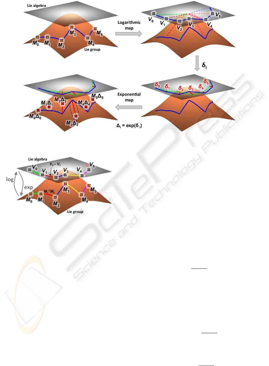
Figure 3: Conceptual view of the change-point detection on SE(3). As discussed in the text, in practice, if the Riemannian

metric is used, the set of ∆

= exp(δ

) does not need to be calculated.

Figure 4: The points M

−1

i+1

∈ SE(3) (assumed to be in

a neighborhood of I

) are mapped onto V

i+1

− V

∈ se(3) by

the logarithmic map. The inverse mapping can be achieved

by the exponential map.

small displacements M

−1

j+1

from the initial ele-

ment M

. Note that we assume these displacements

small enough so that

= log



−1

j+1



(13)

exists. Equation (12) can then be written

∀i ∈ ~1, n − 1, M

= M

i−1

j=0

exp





. (14)

Similarly to the approach presented by (Lee and

Shin, 2002), we construct the following sequence

in se(3): given an initial condition V

, ∀i ∈ ~0, n −

2, V

i+1

= ϕ

(Figure 4). We get the two following

relations for i ∈ ~1, n − 1:

= M

i−1

j=0

exp



j+1

− V



, (15)

and

= V

i−1

j=0

log



−1

j+1



. (16)

4.3 Application of the Mean Filter

The ﬁlter M

is deﬁned so that log(M

−1

)) =

) − V

, which can be written

) = M

exp







2N + 1

k=−N

i+k

− V







. (17)

By following a similar development as in the work of

(Lee and Shin, 2002), we obtain:

) = M

exp



(ϕ

) − ζ

(ϕ

)



, (18)

with

(ϕ

) =

N−1

k=0

N − k

2N + 1

i+k

, (19)

and

(ϕ

) =

N−1

k=0

k + 1

2N + 1

i−N+k

. (20)

CHANGE-POINT DETECTION ON THE LIE GROUP SE(3) FOR SEGMENTING GESTURE-DEFINED SPATIAL

RIGID MOTION

289

The term ζ

(ϕ

) − ζ

(ϕ

) can thus be interpreted as

a diﬀerence of weighted means. Let this diﬀerence of

weighted means be denoted by

= ζ

(ϕ

) − ζ

(ϕ

). (21)

4.4 Change-Point Detection

As previously discussed, the change-points should

correspond to local maximums of the series

(d(M

, M

)))

. Considering the Riemannian dis-

tance, (18) leads to

d(M

, M

)) =



log



−1

)





(ϕ

) − ζ

(ϕ

)



. (22)

Equality (22) shows that the value of M

) does

not need to be explicitly computed. If kδ

is greater

than at any other points in the vicinity of M

, then M

is declared as potentially a change-point. Formally,

this can be expressed as: For a selected n ∈ N

∗

, e.g.,

n = N, if

> max

j,i, j∈~i−n,i+n

kδ

, (23)

then M

is a candidate for a change-point. Such an ap-

proach yields a candidate every 2n points, therefore,

each candidate must be examined for avoiding false

positive. We can adapt the test suggested by (Agar-

wal et al., 2006). For example, given a candidate M

if kδ

> xkζ

(ϕ

, x ∈]0, 1], then M

is declared to

be a valid change-point (the value x have to be empir-

ically selected).

5 RESULTS

In this section, we attempt to evaluate our method.

First, we assess the method based on simulation study.

Then, we conduct a set of experiments using real data

acquired via a motion capture device.

It follows from the previous section that one of

the important step of the detection process consists

in ﬁnding the local maxima of the function η : M

∈

SE(3) 7→

∈ R

(or equivalently, i 7→

). In

practice, a realistic scenario is that the motion is dis-

turbed by noise (e.g., due to motion capture device

imperfection), which consequently, aﬀects the func-

tion η. In order to limit the potential detection er-

rors caused by this noise, we perform two diﬀerent

smoothing ﬁlters. Those ﬁlters are intended to reduce

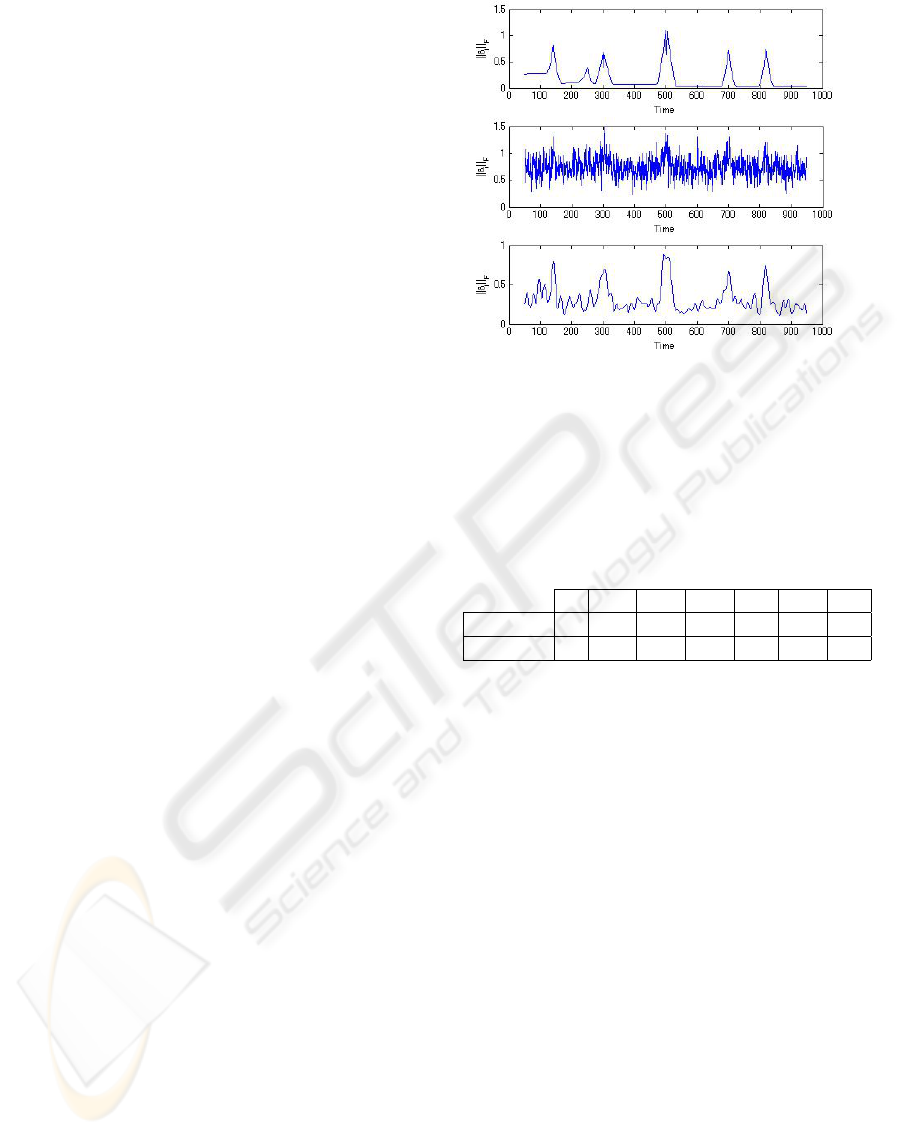
Figure 5: Data smoothing for enhancing the results (these

data are obtained from the original signal depicted in Fig-

ure 6). Plot of the function t 7→

∈ R

without noise

(top), with strong Gaussian noise added to the original sig-

nal (middle), after smoothing both the motion and the func-

tion η itself (bottom).

Table 1: Deﬁnition of the noise level (NL). Both the po-

sition signal and the orientation signal (Figure 6) are dis-

turbed with a Gaussian noise of mean zero and standard de-

viation σ

and σ

, respectively.

0 1 2 3 4 5 6

(cm) 0 0.5 1 1.5 2 2.5 3

(

◦

) 0 2 2.5 5 10 20 40

the high frequency components of the data. There-

fore, the change-points should not be aﬀected (as-

suming a Gaussian noise of mean zero, the response

of the mean ﬁlter M

should remain unchanged af-

ter attenuating the high frequency components due to

noise). Figure 5 illustrates the beneﬁts of this two-

steps smoothing.

First, the motion data is smoothed using an adap-

tation of the orientation ﬁlter suggested by (Lee and

Shin, 2002). Although we have observed that this ﬁl-

ter greatly enhances the motion by signiﬁcantly re-

ducing additive noise, it is not removed.

Second, to avoid the detection of spurious max-

ima, we smooth the function η to attenuate the high

frequency components. This smoothing operation is

performed via the Savitzky-Golay ﬁlter. The choice

of this ﬁlter is motivated by its great property of pre-

serving important features of the signal such as the

extrema and the width of peaks.

GRAPP 2010 - International Conference on Computer Graphics Theory and Applications

290

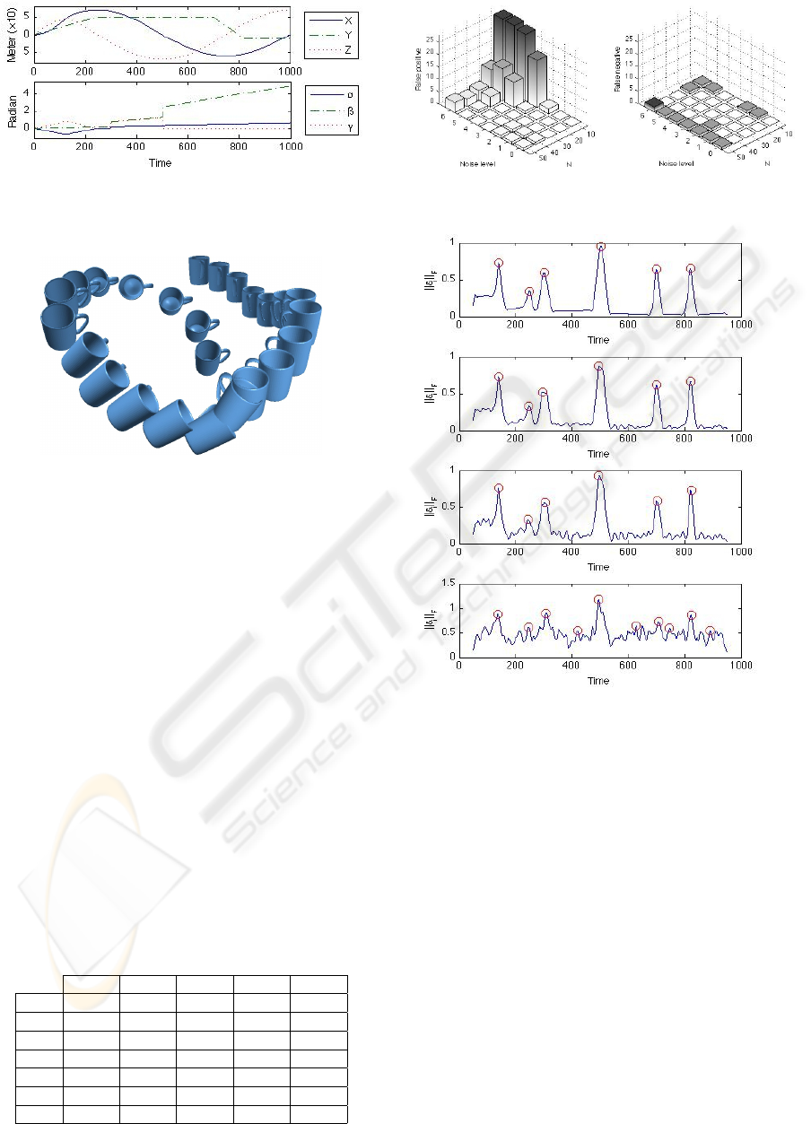
Figure 6: Original signal for generating the simulated mo-

tion. the top graph shows the positions, whereas the bottom

graph gives the orientation (by means of Euler angles).

Figure 7: A teacup displayed at each 40 pose of the motion

generated by the signal shown in Figure 6.

5.1 Synthetic Data

We generate a synthetic motion (M

, . . . , M

1000

). The

original signal is shown in Figure 6, and Figure 7 de-

picts a visual representation by means of a teacup. By

construction, there are a total of six change-points lo-

cated at index 140, 250, 300, 500, 700 and 820.

5.1.1 Eﬀects of Noise Level and Windows Size

We study the eﬀects of both, (i) the noise level, and

(ii) the choice of the window size N, on the change-

point detection results in terms of false positives and

false negatives. Table 1 gives our deﬁnition of seven

noise levels to which we refer to throughout the sim-

ulations (NL 0, . . . , NL 6). A change-point M

considered as discovered when the algorithm ﬁnds a

Table 2: Results of the change-points detection, depending

on the noise level and the window size, in terms of false

positive (FP) and false negative (FN). Each cell gives the

couple (FP, FN).

N = 10 N = 20 N = 30 N = 40 N = 50

NL 0 (0, 0) (0,0) (0, 0) (1, 0) (1, 1)

NL 1 (0, 1) (0, 0) (0, 0) (1, 0) (1, 1)

NL 2 (2, 1) (0, 0) (0, 0) (1, 1) (1, 1)

NL 3 (19, 0) (1, 0) (0,0) (0, 0) (0, 1)

NL 4 (27, 0) (10,0) (0, 0) (0, 0) (0, 1)

NL 5 (28, 1) (13,0) (4, 0) (1, 0) (0, 1)

NL 6 (28, 1) (10,1) (4, 0) (3, 0) (4, 2)

Figure 8: Visual representation of the results summarized

in Table 2.

Figure 9: Plot of the function t 7→

for N = 30 and

(from top to bottom) noise level 0 , 1, 3, 6. The circles

correspond to the detected change-points.

point in its vicinity, i.e., M

n±k

, with k < 10. If sev-

eral points are in the vicinity, then only the nearest is

counted as valid (i.e., the other points are considered

as false positives).

Table 2 summarizes the results for 35 simulations

during which the window size N varies from 10 to 50

by step of 10, whereas the noise level increases from

level 0 to level 6. Figure 8 gives a visual representa-

tion of the same results.

We can observe that when the window size N is

reaching 50, a change-point is systematically missed,

independently of the noise level. This result is actu-

ally expected for the window size becomes larger than

the distance between two subsequent change-points.

Thus, only one will be discovered. At the other ex-

tremity, when N is small, the method is unstable, and

appears to be very sensitive to noise. Especially, a

CHANGE-POINT DETECTION ON THE LIE GROUP SE(3) FOR SEGMENTING GESTURE-DEFINED SPATIAL

RIGID MOTION

291

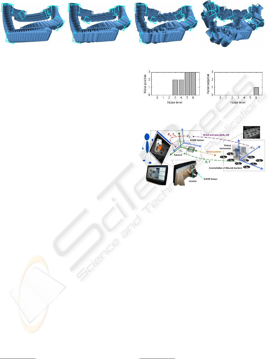
Figure 10: A teacup displayed at each 10 pose of the motion. The noise level is set at (from left to right) 0, 1, 3 and 6. The

cups encapsulated in a frame correspond to the discovered change-points.

large number of false positives are yielded as soon as

the noise level reaches 3. Alternatively, a moderate

window size (e.g., between 30 and 40) provides good

results. When the noise level is high, we can observe

only few false positives.

Figure 9 shows the plots of the function t 7→

for the window size set at 30 and the noise level set

at 0, 1, 3 and 6. Figure 10 gives the corresponding

representation of the motion (via a teacup) in which

the change-point are emphasized.

Globally, the simulation suggests that, assuming

an adequate selection of the window size, one can ex-

pect a low number of false positives and a very low, if

any, number of false negatives.

5.1.2 Comparison Against SST

Singular Spectrum Transform (SST) is a robust

change-point detection method based on the PCA

((Moskvina and Zhigljavsky, 2003), (Ide and Tsuda,

2007)). One of its great advantage compared with

various previous attempts is its capability to be ap-

plied to analyze “complex” data series (in terms of

“shape”) without restrictive assumptions about the

data model. For example, it can deal with data series

for which the distribution depends on the time, such as

arbitrary piecewise-deﬁned functions (e.g., connected

aﬃne segments).

Since SST is designed for manipulating only

scalar time series, to compare the results obtained by

the both SST and our proposed method, ﬁrst, we ap-

ply the SST method to each of the six components

of the signal that served for generating our synthetic

motion (Figure 6), and second, we consolidate the re-

sults to determine the change-points. We use the soft-

ware written by the authors of the algorithm discussed

by (Moskvina and Zhigljavsky, 2003) (which is freely

distributed

). During the experiment we use the set-

ting suggested by the software.

Figure 11 presents the results. We can observe

that the performance, in terms of false positive and

false negative, of both our method and SST are com-

http://www.cardiﬀ.ac.uk/maths/subsites/stats/change-

point

Figure 11: False positive and false negative yielded by the

SST method applied to the signal depicted in Figure 6.

Figure 12: 3D items animation engine.

parable (assuming a proper selection of the window

size N, see Table 2). Both methods yield a limited

number of false positives when the noise level reach a

certain level, with possibly a very few false negatives.

This results should be interpreted loosely, for the SST

algorithm requires an adequate setting of ﬁve parame-

ters. A better tuning of those parameters might lead to

improving the performances. However, we observed

that the setting suggested by the software usually pro-

vide good results.

5.2 Real Data

We have integrated our change-point detection

method into a 3D items animation engine, such as the

one described by (Merckel and Nishida, 2009), which

is an hand-held MR system (Figure 12). It consists of

a tablet PC equipped with a video camera and the IS-

1200 VisTarcker

(Foxlin and Naimark, 2003), which

is a 6-DOF (position and orientation) vision-inertial

tracker.

This engine is intended for providing experts of

Manufactured by InterSense, Inc., http://www.inter-

sense.com

GRAPP 2010 - International Conference on Computer Graphics Theory and Applications

292

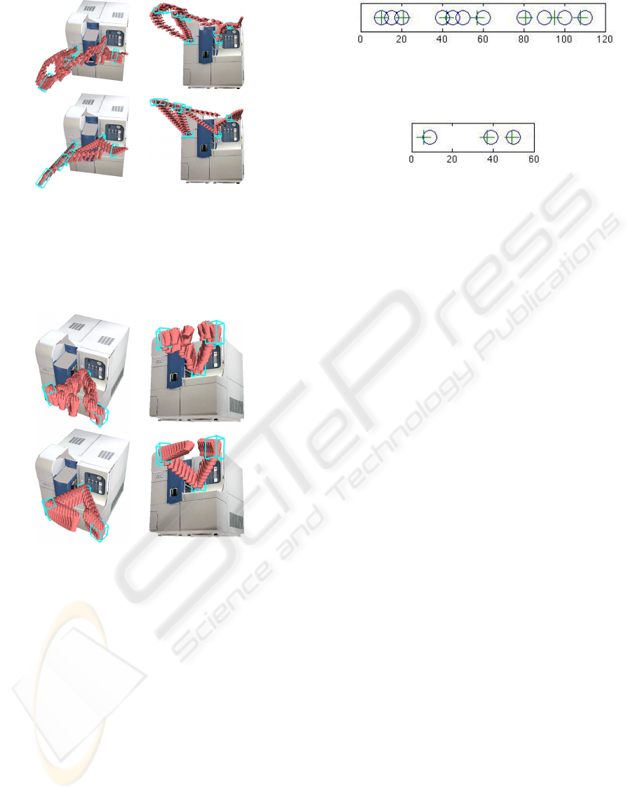
Figure 13: Motion of the pointing-hand in the context of

a virtual instrument. The objective is to push sequentially

two diﬀerent buttons located on the surface of the instru-

ment. The scene is shown from two diﬀerent view-points.

Original user’s inputs (top). Interpolated motion between

change-points (bottom). The hands encapsulated in a frame

correspond to the discovered change-points.

Figure 14: Motion of the picking-hand in the context of a

virtual instrument. The objective is to express that the han-

dle of the front cover must be grasped and pulled. The scene

is shown from two diﬀerent view-points. Original user’s in-

puts (top). Interpolated motion between change-points (bot-

tom). The hands encapsulated in a frame correspond to the

discovered change-points.

complex instruments with an eﬃcient means of com-

municating knowledge, to end-users, about 3D tasks

that must be performed for properly operating the in-

struments. Especially, it allows to animate existing

3D items (CAD models) in the context of a subject

instrument (that can be a physically concrete instru-

ment, or alternatively, a virtual representation). For

animating an items, the user move the tablet PC in the

real-world as if it was the item. The motion is then

captured via the VisTracker. In other words, the en-

gine allows to acquire freehand motion.

Note that the motion is not directly given by the

sensor. As depicted in Figure 12, the motion is de-

Figure 15: Detected change-points in the pointing-hand mo-

tion. The 7 crosses are the ones found using our method,

while the 11 circles are the ones found using the SST

method.

Figure 16: Detected change-points in the pointing-hand mo-

tion. The 3 crosses are the ones found using our method,

while the 3 circles are the ones found using the SST method.

ﬁned by the time sequence of poses R and T (i.e.,

the camera pose). These poses are also required for

registering the virtual objects (the item being animat-

ing and the virtual instrument) in the current scene.

The VisTarcker measures the coordinates (X, Y, Z)

and the orientation (yaw, pitch and roll) of the sen-

sor reference frame R

in the world reference frame

. The relative position T

and orientation R

the VisTracker (R

) and the video camera (R

) need

to be known to compute the camera pose. To deter-

mine this transformation, we perform an initial cal-

ibration process that consists in computing n poses

, T

) from diﬀerent viewpoints using a purely opti-

cal method (chessboard pattern recognition), simulta-

neously, recording the sensor data (R

s,i

, T

s,i

), and ﬁ-

nally, ﬁnding the R

and T

that minimized the cost

function

i=1

(kR

− R

s,i

k + kT

− (R

s,i

+ T

)k).

Figure 13 and 14 show the captured motion for

two diﬀerent scenarios. In the ﬁrst one (Figure 13),

the user is moving a pointing-hand model to sequen-

tially push two diﬀerent buttons. In the second one

(Figure 14), the user is moving a picking-hand model

for expressing a situation in which the handle of a

cover has to be grasp and pulled. In both ﬁgures,

the top row depicts the original user’s input, while

the bottom row represents an enhanced version. We

can observed that the discovered change-points are

pertinent in the sense that, in both cases, the mo-

tion segmentation correspond to the user’s intent (the

buttons are pushed, and the handle is grasped and

pulled), and consequently, the motion is successfully

and greatly enhanced (e.g., the unintended “jerky”

movements are removed). The performed interpola-

tion here consists of a naive “screw-motion” joining

the change-points and ignoring the all other points

input by the user. To better represent the user’s in-

tention, a more elaborated method, such as the one

discussed by (Hofer and Pottmann, 2004), should be

considered.

For comparison, we have performed the SST

CHANGE-POINT DETECTION ON THE LIE GROUP SE(3) FOR SEGMENTING GESTURE-DEFINED SPATIAL

RIGID MOTION

293

method to the 6 components of the motion signal

output by the VisTracker. In the ﬁrst scenario, we

have discovered a total of 7 change-points using our

method, whereas the SST method has yielded 11

change-points. Figure 15 shows the relative distri-

butions of those two sets of points. One can ob-

served that the two results are, to a fairly large ex-

tent, well-correlated. Although the SST method has

discovered 4 points more than our method, the rela-

tive distributions (Figure 15) suggests that we could

“cluster” together the 11 points in a way that cor-

respond to the 7 points discovered by our approach.

Especially, regarding that the 11 points are an in-

terpolation through consolidation of the SST results

independently obtained from the 6 signals received

from the VisTracker. A change in one of the sig-

nal at time t, and a change in another signal at time

t +  (with  small), might have the same cause. Even

though, two change-points may be discovered. Our

method searches for changes in a particular mixture

of the 6 signals (that leads to a series in SE(3)), which

may yield a single change at, e.g., t + /2. This phe-

nomenon is unlikely to occur in the synthetic data, for

the cause leading to a change is, by construction, well

synchronized between the signals. Moreover, the ar-

tiﬁcial noise follows a neat Gaussian distribution (in

practice, the stochastic imperfection of the real data

due to various causes is unlikely to follow a perfect

Gaussian law).

Considering the second scenario, Figure 16 shows

that the both methods give comparable results. Only

a slight shift in the change-point positions can be ob-

served between the two approaches.

6 CONCLUSIONS

We have proposed a method for detecting change-

points in rigid-body motion time series. This method

can be regarded as an adaptation of the diﬀerence of

means method to time series in SE(3). It is based on

the key observation that the absolute gain of the mean

ﬁlter yields a local maximum when a change occurs.

By exploiting this result and the particular Lie group

structure of SE(3), we have shown that the change-

points in SE(3) can be discovered in its Lie algebra

se(3) through the following process: The initial time

series in SE(3) is transformed in a corresponding time

series in se(3) (via logarithmic mapping). Then for

each point in the vector space se(3), we calculate the

norm of the diﬀerence between a weighted mean of

the point to the left and a weighted mean of the point

to the right. Finally, the potential change-points cor-

respond to the maximum values.

A set of evaluations has been conducted showing

that, assuming an adequate parameter setting (mainly

the window size of the mean ﬁlter), the method should

yield a low number of false positives and a very low,

if any, number of false negatives.

REFERENCES

Agarwal, M., Gupta, M., Mann, V., Sachindran, N., Aner-

ousis, N., and Mummert, L. (2006). Problem de-

termination in enterprise middleware systems using

change point correlation of time series data. In

2006 IEEE/IFIP Network Operations and Manage-

ment Symposium NOMS 2006, pages 471–482. IEEE.

Basseville, M. and Nikiforov, I. V. (1993). Detection of

Abrupt Changes - Theory and Application. Prentice-

Hall, Inc, Englewood Cliﬀs, N.J.

Buss, S. R. and Fillmore, J. P. (2001). Spherical averages

and applications to spherical splines and interpolation.

ACM Trans. Graph., 20(2):95–126.

Courty, N. (2008). Bilateral human motion ﬁltering. In the

16th European Signal Processing Conference, Lau-

sanne, Switzerland.

Drummond, T. and Cipolla, R. (2002). Real-time visual

tracking of complex structures. IEEE Transactions on

PAMI, 24:932–946.

Fiorentino, M., Monno, G., Renzulli, P. A., and Uva,

A. E. (2003). 3D sketch stroke segmentation and ﬁt-

ting in virtual reality. In International conference on

the Computer Graphics and Vision, pages 188–191,

Moscow, Russia.

Fletcher, P. T., Lu, C., and Joshi, S. (2003). Statistics of

shape via principal geodesic analysis on lie groups.

In IEEE Conference on Computer Vision and Pattern

Recognition, pages 95–101. IEEE Comput. Soc.

Foxlin, E. and Naimark, L. (2003). Vis-tracker: A wear-

able vision-inertial self-tracker. Virtual Reality Con-

ference, IEEE, 0:199.

Gombay, E. (2008). Change detection in autoregressive

time series. Journal of Multivariate Analysis, 99:451–

464.

Govindu, V. M. (2004). Lie-algebraic averaging for globally

consistent motion estimation. In IEEE Conference on

Computer Vision and Pattern Recognition, pages 684–

691. IEEE Comput. Soc.

Grassia, F. S. (1998). Practical parameterization of rotations

using the exponential map. journal of graphics, gpu,

and game tools, 3(3):29–48.

Hofer, M. and Pottmann, H. (2004). Energy-minimizing

splines in manifolds. ACM Transactions on Graphics,

23(3):284–293.

Huang, J.-S. (2000). Introduction to Lie Groups, chapter 7,

pages 71–89. World Scientiﬁc Publishing Company.

Ide, T. and Inoue, K. (2005). Knowledge discovery from

heterogeneous dynamic systems using change-point

correlations. In SIAM International Conference on

Data Mining, pages 571–576.

GRAPP 2010 - International Conference on Computer Graphics Theory and Applications

294

Ide, T. and Tsuda, K. (2007). Change-point detection us-

ing krylov subspace learning. In SIAM International

Conference on Data Mining, pages 515–520.

Kawahara, Y. and Sugiyama, M. (2009). Change-point de-

tection in time-series data by direct density-ratio es-

timation. In SIAM International Conference on Data

Mining.

Lee, J. and Shin, Y. S. (2002). General construction of time-

domain ﬁlters for orientation data. IEEE Transactions

on Visualization and Computer Graphics, 8:119–128.

Merckel, L. and Nishida, T. (2009). Towards expressing

situated knowledge for complex instruments by 3D

items creation and animation. In The 8th International

Workshop on Social Intelligence Design, pages 301–

315, Kyoto, Japan.

Moskvina, V. and Zhigljavsky, A. (2003). An algorithm

based on singular spectrum analysis for change-point

detection. Communications in Statistics: Simulation

and Computation, 32:319–352.

Qin, S.-F., Wright, D. K., and Jordanov, I. N. (2001). On-

line segmentation of freehand sketches by knowledge-

based nonlinear thresholding operations. Pattern

Recognition, 34:1885–1893.

Selig, J. M. (2005). Lie Algebra, chapter 4, pages 51–

83. Monographs in Computer Science. Springer New

York, New York.

Sezgin, T. M. and Davis, R. (2004). Scale-space based fea-

ture point detection for digital ink. In Making pen-

based interaction intelligent and natural, AAAI fall

symposium.

Srivastava, A. and Klassen, E. (2002). Monte Carlo extrin-

sic estimators of manifold-valued parameters. IEEE

Transactions on Signal Processing, 50(2):299–308.

Stuelpnagel, J. (1964). On the parametrization of the three-

dimensional rotation group. SIAM Review, 6:422–

430.

Subbarao, R. and Meer, P. (2006). Nonlinear mean shift

for clustering over analytic manifolds. In Computer

Vision and Pattern Recognition, pages 1168–1175.

IEEE.

Tuzel, O., Subbarao, R., and Meer, P. (2005). Simultaneous

multiple 3d motion estimation via mode ﬁnding on lie

groups. In Tenth IEEE International Conference on

Computer Vision, pages 18–25. IEEE.

van Dam, A. (1997). Post-wimp user interfaces. Communi-

cations of the ACM, 40(2):63–67.

Zefran, M., Kumar, V., and Croke, C. (1998). On the gen-

eration of smooth three-dimensional rigid body mo-

tions. IEEE Transactions on Robotics and Automa-

tion, 14:576–589.

CHANGE-POINT DETECTION ON THE LIE GROUP SE(3) FOR SEGMENTING GESTURE-DEFINED SPATIAL

RIGID MOTION

295