UNDERSTANDING PHOTOGRAPHIC COMPOSITION THROUGH
DATA-DRIVEN APPROACHES
Dansheng Mao, Ramakrishna Kakarala, Deepu Rajan
School of Computer Engineering, Nanyang Technological University, Singapore
Shannon Lee Castleman
School of Arts, Design and Media, Nanyang Technological University, Singapore
Keywords:
Computational Aesthetics, Computer vision, Machine learning, Visual perception, Saliency model.
Abstract:
Many elements contribute to a photograph’s aesthetic value, include context, emotion, color, lightness, and
composition. Of those elements, composition, which is how the arrangement of subjects, background, and
features work together, is both highly challenging, and yet amenable, for understanding with computer vision
techniques. Choosing famous monochromic photographs for which the composition is the dominant aesthetic
contributor, we have developed data-driven approaches to understand composition. We obtain two novel
results. The first shows relationships between the composition styles of master photographers based on their
works, as obtained by analyzing extracted SIFT features. The second result, which relies on data obtained from
eye-tracking equipment on both expert photographers and novices, shows that there are significant differences
between them in what is salient in a photograph’s composition.
1 INTRODUCTION
There are many contributors to aesthetics in photogra-
phy, including color, lightness, emotion, context, and
composition. What is interesting about composition
from a computer vision perspective is that it is highly
challenging to understand, and yet, being based on
geometrical arrangements of subjects, features, and
background, also amenable to image analysis. Com-
position has traditionally been studied by qualitative
means (Zakia, 2007). In this paper, we take a data-
driven approach, using both feature extraction with
computer vision techniques and statistical analysis of
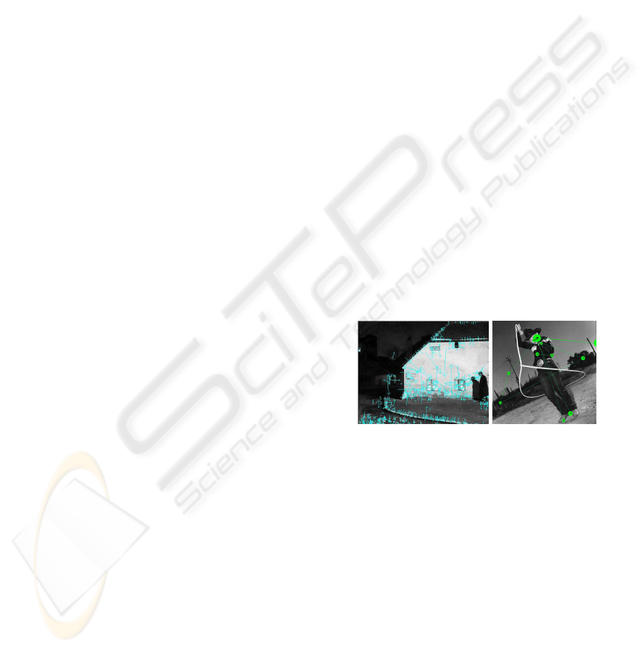
eye-tracking data. Figure 1 shows, for illustrative pur-
poses, the two types of data that we use.
Much prior work in computational aesthetics re-
lated to our paper is devoted to studying paint-
ings, rather than photographs. Taylor et al.’s (Taylor
et al., 1999) fractal analysis of Jackson Pollock’s drip
paintings, later disputed by Jones-Smith and Mathur
(Jones-Smith and Mathur, 2006), was followed by
Rockmore et al (Lyu et al., 2004), who used multi-
resolution visual analysis of brush strokes to iden-
tify how many apprentices worked on a master paint-
ing. Bressan et al (Bressan et al., 2008) also work on
(a) Scale invariant fea-
tures.
(b) Human fixation
locations.
Figure 1: Examples of the two data types used in this paper:
extracted SIFT features are shown in (a) on a photograph by
Andre Kertesz, and eye-tracking data are shown in (b) on a
photograph by Mary Ellen Mark (Please see colour images
in PDF).
paintings, and provide a multidimensional scaling ap-
proach to describing the similarities between painters
based on their works. Much work has been devoted to
measuring facial attractiveness from images, see (Ka-
gian et al., 2006) and the references therein. Aesthetic
analysis of photographs from user ratings has been
discussed by Datta et al(Datta et al., 2006). In their
approach, the aesthetic value of an image is predicted
by a classifier trained on image ratings from users on
such sites as Photo.net.
While this approach is useful to predict ratings
425
Mao D., Kakarala R., Rajan D. and Lee Castleman S. (2010).
UNDERSTANDING PHOTOGRAPHIC COMPOSITION THROUGH DATA-DRIVEN APPROACHES.
In Proceedings of the International Conference on Computer Vision Theory and Applications, pages 425-430
DOI: 10.5220/0002842104250430
Copyright
c
SciTePress
with a particular group of users, it does not illuminate
the role of composition. The black and white pho-
tographs of the master photographers known for their
strong composition, such as Henri Cartier-Bresson,
would not rate highly with that approach. Recent
work on photographic visual saliency by Judd et al.
(Judd et al., 2009) uses eye-tracking data, which is
fed as ground-truth data into a SVM trainer for a
saliency predictor. However, their study did not fo-
cus on photographs known for composition, nor did it
distinguish expert photographers from novices, both
of which we do in this paper.
Our work looks into the relationship of photo-
graphic composition among master photographers,
and also examines the differences in saliency between
expert photographers and novices. The relationships
in composition style of eight master photographers is
described with the aid of multi-dimensional scaling.
Specifically, the similarity between any two photogra-
phers is measured with the Fisher kernel method (Per-
ronnin and Dance, 2007), which uses features extractd
from their photographs and modelled by a Gaussian
mixture distribution. We also describe differences be-
tween what experts find salient in a composition and
what novices do by analyzing data obtained with eye-
tracking equipment. We use receiver operating char-
acteristic (ROC) analysis to describe how consistent
novices are with each other, how consistent experts
are, and how well each group predicts the other.
2 PHOTOGRAPHER DATASET
We collected 106 monochromic photographs of 8 fa-
mous photographers, who are known for their com-
position styles, by scanning images from published
books. The images have about 1 megapixel per im-
age. We call this the Π dataset. Another dataset,
denoted Ω, has 19 photographs, each with resolu-
tion of around 3K pixels per image, was collected
from the Microsoft Bing image search engine to make
sure each selected photographer has at least 15 pho-
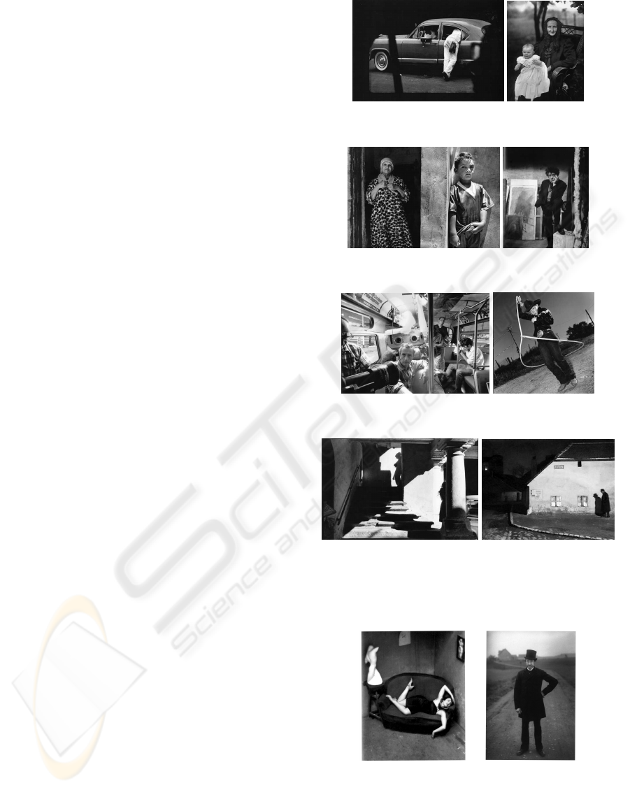
tographs. Figure 2 gives a sample photograph of the
each photographer used.
Since we reduce the photograph size prior to
feature-based data analysis to avoid redundant fea-
tures being extracted, the evaluation for our feature-
based approach involved both Π and Ω. For the exper-
iment with eye-tracking equipment describe in Sec-
tion 4, the photographs shown to the user for appre-
ciation on a 1024 × 768 monitor were from Π, and
were scaled equally in each dimension in order to fit
the full screen.
(a) W. Eugene Smith. (b) August
Sander.
(c) Sebastiao Salgado. (d) Robert
Doiseneau.
(e) Bruce Davidson. (f) Mary Ellen
Mark.
(g) Henri Cartier Bresson. (h) Andre Kertesz.
Figure 2: Sample photographs from the dataset. Though
the resolutions varies with different photographs, they have
been resized with aspect ratios preserved for viewing here.
(a) “Dancer” by An-
dre Kertesz.
(b) “Farmer” by
August Sander.
Figure 3: The most dissimilar pair of photographs in com-
position style from the 8 different photographers in our
dataset. Note that the ”Dancer” photograph is primarily hor-
izontal, while the ”Farmer” is vertical.
VISAPP 2010 - International Conference on Computer Vision Theory and Applications
426
3 UNDERSTANDING WITH
FEATURE-BASED DATA
Photographic composition relies on arrangements of
attributes (colors, texture) and features (lines, curves,
faces) that are identifiable by computer vision tech-
niques. In computer vision, the bag of words (BoW)
model with the attributes and features is a popular rep-
resentation for image categorization. The main idea is
to characterize an image with the histogram of the vi-
sual words, and the histogram vector could be used
with any discriminative classifier or categorizer. A
drawback of the BoW method is that the computa-
tional complexity is often high, since it relies on local
features extracted from the image.
3.1 Fisher Kernel based Image
Representation
Within the field of pattern classification, the Fisher
kernel is a powerful framework which combines as-
pects of generative and discriminative approaches
(Jaakkola and Haussler, 1998). Let p be a pdf which
models the distribution of the low level features in any
image, and let λ denote the parameters that the model
relies on. Let X = {x
t
, t ∈ [1, T]} denote a set of low-
level features extracted from an image. The features
are then represented as the following gradient vector:
G
X
= ∇
λ
log p(X|λ) = ∇
λ
Σ
T
t=1
log p(x
t
|λ). (1)
In our case, p is a Gaussian Mixture Model (GMM)
trained on the set of photographs that we chose. Intu-
itively, the gradient G
X
of the log-likelihood describes
the direction in which parameters should be modified
to best fit the data. It transforms a variable length
sample X into a fixed length vector whose size is only
dependent on the number of parameters in the pdf
model. Hence, G
X
can be fed into any discrimina-
tive classifier. For those classifiers that measure the
similarity by the inner product technique, it is neces-
sary to normalize the input vector. In (Jaakkola and
Haussler, 1998), the Fisher information matrix F
λ
(X)
is defined for that purpose as follows (with
′
denoting
transpose):
F
λ
(X) = E
X
[∇
λ
log p(X|λ)∇
λ
log p(X|λ)
′
]. (2)
Because of the cost associated with its composition
and inversion of the Fisher information matrix, F
λ
(X)
is often approximated by the identity matrix. We use
the diagonal approximation derived in (Perronnin and
Dance, 2007). Then the similarity between vectors
G
X
and G
Y
can be defined as,
(a) “China” by Sebastiao Sal-
gado.
(b) “Spain” by W. Eu-
gene Smith.
Figure 4: The most similar pair of photographs in composi-
tion style from the 8 different photographers in our dataset.
S
XY
= G
′
X
F
−1
λ
G
Y
. (3)
In order to apply the Fisher kernel method, we need
to define which features are relevant to photographic
composition. Scale-invariant features (SIFT features)
have previously been shown to be useful in judging
similarity between painters (Bressan et al., 2008). We
use them as local feature vectors in our experiment.
SIFT features extract local maxima or minima from a
Gaussian pyramid as key points, and describes each
with a local histogram of orientation, which is robust
to rotation (Lowe, 2004). The features use a thresh-
olded gradient for stability under lighting adjustment.
3.2 Photographers Relationship Graph
In this section, our goal is to build a straightforward
method for visualizing the relationship amongs mas-
ter photographers. A relationship graph is constructed
according to their similarity measurements by using
multi-dimensional scaling. The more similar two
photographers are, the closer they are located on the
graph, and vice versa.
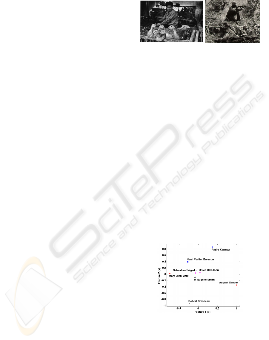
Figure 5: Photographers relationship graph, where prox-
imity indicates similarity. The photographers Doisneau,
Kertesz, Mark have distinctive styles, which agrees with
their positioning in this graph. Henri Cartier-Bresson,
whose work influenced many, is near the central locus of
Salgado, Davidson, and Smith.
Before feeding the SIFT feature vectors into
a GMM trainer (which uses the expectation-
UNDERSTANDING PHOTOGRAPHIC COMPOSITION THROUGH DATA-DRIVEN APPROACHES
427
maximization algorithm) and Fisher kernel similar-
ity measuring function, principal component analysis
(PCA) is applied to reduce the feature vector dimen-
sion. Gradient vectors are computed according to the
equation (1). Then the similarity of all the photograph
pairs in the database can be obtained by the equation
(3). Hence, a symmetric similarity matrix for pho-
tographs, denotedC, is constructed. For the similarity
of the photographers pair, we use corresponding en-
tries fromC. Given photographers A and B, their sim-
ilarity is obtained by summing all entries in C with
photographs from A and B. Obviously, the 8× 8 sim-
ilarity matrix S is also symmetric. Matrix S is nor-
malized to avoid the bias effect due to the different
number of photographs for each author.
To visualize the photographers relationship, we
applied a multidimensional scaling algorithm (van der
Heijden et al., 2004) to map the 8 photographers into
a two-dimensional space. Figure 5 shows the result.
3.3 Results and Discussions
In order to demonstrate the plausibility of using SIFT
features with Fisher kernel representations in deter-
mining composition, we exhibit the most distinctive
and most similar works that belongs to the different
photographers in Figure 3 and Figure 4. The compo-
sition of Figure 3(a) gives strong horizontal feelings
from both the long chair and the lying dancer while
Figure 3(b) gives strong vertical feelings from both
the farmer and the road. For the distribution of the
lightness, Figure 3(a) arranges the dark region in the
ceiling and relative bright regions in the other three
margins. On the contrary, Figure 3(b) arranges the
bright region in the sky and relative dark regions in
the other three margins. Studying the most similar
image pair, both Figure 4(a) and Figure 4(b) are com-
posed with the two objects in the center, where are
upright while the lower objects lie to the right side, ar-
ranged along a vertical line. The backgrounds in both
images are “messy”, which makes the foreground ob-
jects stand out. For the lightness distribution, both
photos make the lower object brighter than the upper
object and let the upper corners be relatively lighter
than the bottom corners.
Figure 5 shows the overall photographer relation-
ship graph obtained through multi-dimensional scal-
ing. Here, proximity indicates similarity. The results
show that certain photographers, such as Mary Ellen
Mark or Andre Kertesz, are “iconoclasts”. Mark is
known for challenging conventions by using oblique
view points and framing. Andre Kertesz’s composi-
tions are also distinctive, in that he organizes subjects
in triangular groupings. Similarly we can comment
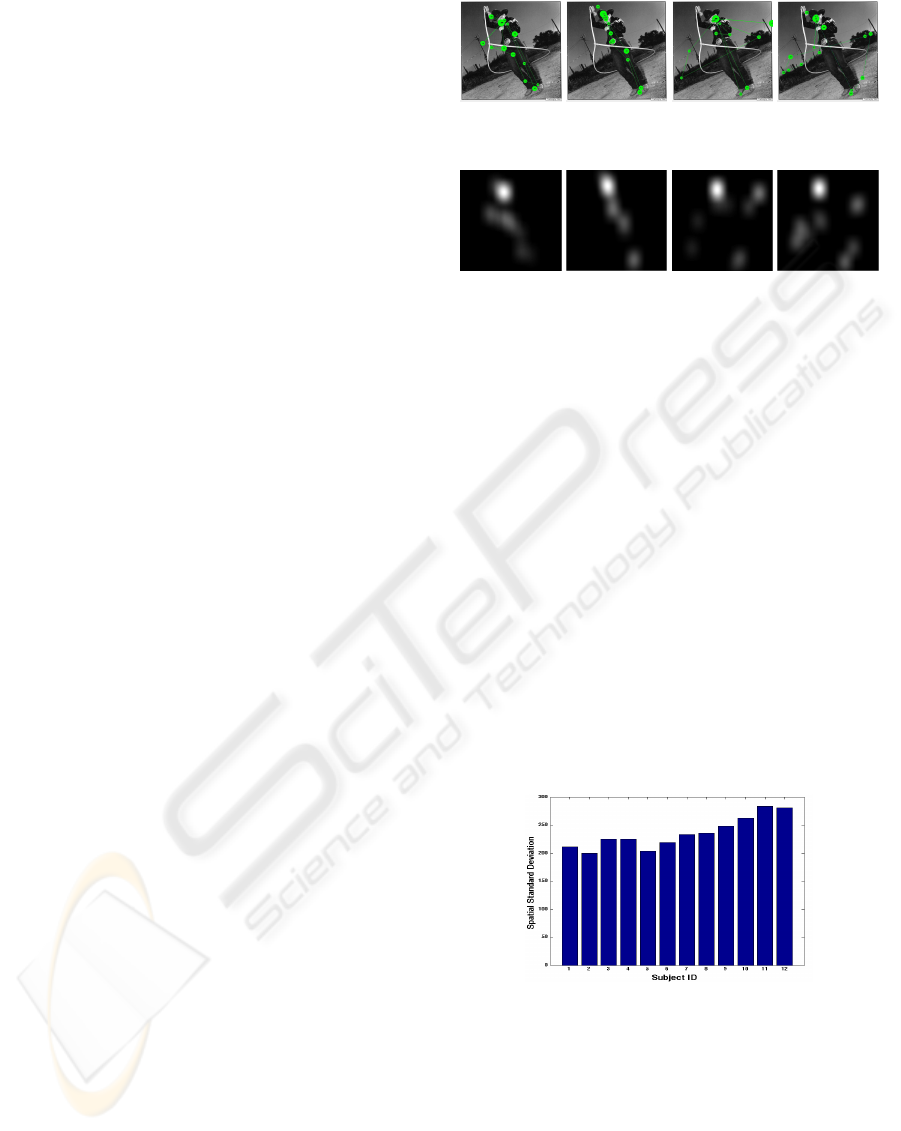
(a) Gaze plot
of novice A.
(b) Gaze plot
of a novice B.
(c) Gaze plot
of expert A.
(d) Gaze plot
of expert B.
(e) Saliency
map of 6(a).
(f) Saliency
map of 6(b).
(g) Saliency
map of 6(c).
(h) Saliency
map of 6(d).
Figure 6: Results obtained from eye-tracking of expert pho-
tographers, and their corresponding saliency maps.
on the distinctiveness of August Sander, who tends to
put his subjects in the center, almost crowding them
in, and Robert Doisneau, whose images often con-
tain humour found in street scenes in Paris. Note also
that Henri Cartier-Bresson, a very influential photog-
rapher, appears near the center, a reasonable outcome
given that others are known to have been influenced
by him. The analysis found Sebastiao Salgado, Bruce
Davidson and W. Eugene Smith to have similar com-
position styles, which agrees with our visual exami-
nation of the photographs.
4 UNDERSTANDING WITH
BEHAVIORAL DATA
Figure 7: Spatial standard deviations of fixation locations of
individual subjects. Bar 1
st
to bar 10
th
are the photographic
novice subjects and the rest are from the expert subjects.
Composition is often considered the art of guiding the
viewer’s eye. In order to understand how composi-
tion affects viewing, we used eye-tracking equipment
to examine visual fixation with both novice and expert
photographers. The consistency of normal human fix-
ations over an image has been investigated by Judd et
al. (Judd et al., 2009). They show that a strong bias
VISAPP 2010 - International Conference on Computer Vision Theory and Applications
428
exists for human fixations to be near the center of the
image, and also conclude that the saliency map from
one user can predict the ground truth fixation of all
users remarkably well. As the fixations have a strong
bias towards the center, Judd et al. show that a Gaus-
sian “blob” predicts the ground truth saliency map
reasonably well. However, they do not consider pos-
sible differences between photographic experts and
novices. We exlored this issue with our subjects.
Our experiments were carried out as follows. We
invited 10 novices and also 2 professional photogra-
phers to participate our experiments. (One of the ex-
pert photographers is a co-author of this paper.) We
set up a slide show of 30 selected photographs from
the Π database, each photograph displayed for 5 sec-
onds. The transition between photographs is filled
with 3 seconds of neutral gray image. We used a Tobii
T-60 eye-tracker to obtain the data.
4.1 The Observations of Eye Fixation
Figure 6(a) and 6(b) are the gaze plots of the novices
on the photograph ”Cowboy” by Mary Ellen Mark,
while Figure 6(c) and 6(d) are the gaze plots from
expert photographers on the same photograph. The
corresponding saliency maps are also shown in the
same columns. The saliency maps are calculated by
convolving a Gaussian kernel on the binary fixation
maps, which in turn are obtained from the gaze plots
by setting the spot size radius to be the square root of
the gaze duration (milliseconds) at that location.
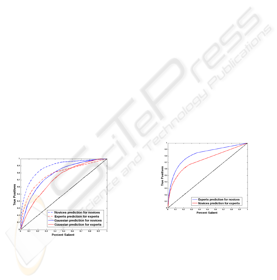
Figure 8: ROC curves for illustrating the performances of
the human prediction and Gaussian blob prediction. We see
that novices are much more consistent in gaze than experts,
and are also much better predicted by a Gaussian blob than
experts.
Observing the gaze plots, we noticed that the gaze
plot of the novice subject is typically concentrated on
the foreground object, and less likely to wander to
the background. For the experts, however, the se-
quence of gazes goes through both foreground and
background, and often wanders to the borders. For
example, they check the symmetry in the composi-
tion evident in the telephone poles around the “Cow-
boy” in the photograph. Therefore, the spatial distri-
bution of gaze plot of the novices are centralized in
the foreground region, while the gaze plots of experts
are more sparse. In the saliency maps, they have many
intersections. In particular, the pixels that have high
saliency are almost located in the same region, sug-
gesting that novices and experts could be predicted
by each other.
To check whether expert photographershave more
dispersed gaze than novices, we computed the spatial
standard deviations of fixation locations over all pho-
tographs. The resuls are plotted in Figure 7. In the
chart, the 1
st
to 10
th
bars belong to novices and the
rest are from experts, showing that experts do gaze
over more of the image than novices.
4.2 Analysis of Eye Fixation Data
We analyzed the fixation data obatined from novices
and experts to see what may be predicted of the two
different groups. Two kinds of predictions are studied
in this paper: human prediction and Gaussian blob
prediction. Human prediction is based on hypothesis
that each group is consistent, and the Gaussian blob
prediction is based on the hypothesis that human fix-
ation is centralized on foreground objects.
Figure 9: ROC curves show that saliency map of novices
is better predicted by experts (blue curve) than vice versa
(red).
In the human prediction experiment, we treat the
saliency map from the fixation locations of one user
in the group as a binary classifier on every pixel in
the photograph. As in Judd et al. (Judd et al., 2009),
the saliency maps are thresholded at a level so that
a given percent of the image pixels are classified as
fixated, and the rest are classified as not fixated. Hu-
man fixations from the other users in the same group
are ground truth fixations. The threshold is varied to
sweep out an ROC curve. The x-axis of the ROC
UNDERSTANDING PHOTOGRAPHIC COMPOSITION THROUGH DATA-DRIVEN APPROACHES
429

curve is the percentage of the image pixels classified,
while the y-axis is the percentage of true fixations that
are classified. We obtained the ROC for each user
in a group and averaged the results within a group.
For the Gaussian blob prediction, we take the accu-
mulated fixation map of users in the group, and fit it
to a circularly-symmetric two-dimensional Gaussian
distribution by matching mean and variance.
Figure 8 shows the prediction performances by the
ROC curves for the both novices and experts. The
dashed curves illustrate the human prediction perfor-
mance while the continuous curves show the Gaus-
sian blob prediction performance. Obviously, the fix-
ation locations of a novice predict those of another
novice much better than one of the experts predicts
another expert. It means the eye fixation of novices
has higher consistency than experts. That is per-
haps because expert photographers put their training
and experience in the appreciation of photographs,
whereas novices tend to look at the obvious in pho-
tographs. From the Gaussian blob prediction result,
we can see the fixation map of novices are more cen-
tral, usually the location of foreground objects. From
the characteristics of the ROC curve, human predic-
tion performs better on novices than experts, and the
same conclusion holds for Gaussian blob prediction.
As mentioned previously, the most salient regions
of the novices usually intersect with experts’ most
salient regions. To examine that effect statistically,
we used each individual user in one group to predict
another user in the other group. The averaged inter-
group prediction ROC curves is shown in Figure 9. It
shows that the prediction of the novice fixation loca-
tion by a master fixation location is much better than
the prediction of a master by a novice. The result may
be understood by noting that the salient region in pho-
tograph for a novice is usually the foreground region,
while the expert considers both foreground and back-
ground regions.
5 CONCLUSIONS
This paper presents two data-driven approaches for
understanding the photographic compositions. The
first is a feature-based method, in which we trained
a GMM model for SIFT features extracted from
monochromic photographs from master photogra-
phers. The similarity of each image pair is mea-
sured by evaluating the gradients of log-likelihood of
the GMM with weighting given by the Fisher matrix.
Then a photographers relationship graph is obtained
by using multi-dimensional scaling. In the second ap-
proach, we used gaze plots measured by eye-tracking
equipment. In that data, the prediction performanceof
both humans and Gaussian blobs are evaluated with
the help of ROC metric. We find that eye fixations
of the novices are much more consistent than those
of expert photographers, and that experts predict the
novices much better than the reverse case. In fu-
ture work, we will examine whether SIFT features
are the best for understanding composition, and study
eye-tracking with “bad” compositions by novices as
judged by experts.
REFERENCES
Bressan, M., Cifarelli, C., and Perronnin, F. (2008). An
analysis of the relationship between painters based on
their work. In ICIP, pages 113–116.
Datta, R., Joshi, D., Li, J., and Wang, J. Z. (2006). Studying
aesthetics in photographic images using a computa-
tional approach. In Proc. ECCV, pages 7–13.
Jaakkola, T. and Haussler, D. (1998). Exploiting generative
models in discriminative classifiers. In In Advances
in Neural Information Processing Systems 11, pages
487–493. MIT Press.
Jones-Smith, K. and Mathur, H. (2006). Fractal analysis:
Revisiting pollock’s drip paintings. Nature, pages E9–
E10.
Judd, T., Ehinger, K., Durand, F., and Torralba, A. (2009).
Learning to predict where humans look. In ICCV.
Kagian, A., Dror, G., Leyvand, T., Cohen-Or, D., and Rup-
pin, E. (2006). A humanlike predictor of facial attrac-
tiveness. In NIPS, pages 649–656.
Lowe, D. G. (2004). Distinctive image features from scale-
invariant keypoints. International Journal of Com-
puter Vision, 60:91–110.
Lyu, S., Rockmore, D., and Farid, H. (2004). A digital tech-
nique for art authentication. Proceedings of the Na-
tional Academy of Sciences, 101(49):17006–17010.
Perronnin, F. and Dance, C. R. (2007). Fisher kernels on vi-
sual vocabularies for image categorization. In CVPR.
Taylor, R. P., Micolich, A. P., and Jonas, D. (1999). Fractal
analysis of pollock’s drip paintings. Nature, 399:422.
van der Heijden, F., Duin, R., de Ridder, D., and Tax, D.
M. J. (2004). Classification, Parameter Estimation
and State Estimation. Wiley.
Zakia, R. (2007). Perception and imaging: photography–a
way of seeing. Elsevier Science Ltd.
VISAPP 2010 - International Conference on Computer Vision Theory and Applications
430
