
EMBEDDING HIERACHICAL DEFORMATION WITHIN A
REALTIME SCENE GRAPH
A Simple Approach for Embedding GPU-based Realtime Deformations using
Trilinear Transformations Embedded in a Scene Graph
M. Knuth, J. Kohlhammer
Fraunhofer Institute for Computer Graphics Research (IGD), Germany
A. Kuijper
Interactive Graphics Systems Group, TU Darmstadt, Germany
Keywords:
Realtime rendering, Deformation, Scenegraphs, GPU.
Abstract:
Scene graphs are widely used as a description of spatial relations between objects in a scene. Current scene
graphs use linear transformations for this purpose. This limits the relation of two objects in the hierarchy to
simple transformations like sheer, translation, rotation and scaling. In contrast to this, we want to represent
and control deformations that result from propagating the dynamics of objects to deformable attached objects.
Our solution is to replace the linear 4x4 matrix-based transformation of a scene graph by a more generic
trilinear transformation. The linear transformation allows the composition of the transformation hierarchy
into one transformation. Our approach additionally allows the handling of deformations on the same level.
Building on this concept we present a system capable of real-time rendering. The computations of the applied
deformations of the scene graph are performed in real-time on the GPU. We allow the approximation of
arbitrary nonlinear transformations and deformations by utilising grids of trilinear transformations in our
system. As an application we show geometric attachments on deformable objects and their deformation on a
scene graph level.
1 INTRODUCTION
In complex scenes it is useful to organise the scene
elements in a hierarchy to achieve a structured scene
management. These scene graphs bundle the objects
in groups and assign spatial relations between them.
This allows a simple approach for the grouping and
construction of larger building blocks, which are rep-
resented by linear transformations. While grouping
relates objects spatially to each other, it is sometimes
necessary to attach an object to the surface of another
object. For this problem the grouping mechanism of
the graph is sufficient, as long the surface of the ob-
ject does not change. An example of such a scenario
is the attachment of accessories on a piece of gar-
ment or an animated 3D avatar or object in a computer
game. In this cases it is necessary to update the acces-
sories’ transformation in respect to the surface of the
animated object.
If the accessory has a static nature (for example
a button) this problem can be still solved using a lin-
ear transformation system. However, it is often nec-
essary to attach elements on several points on a de-
forming object. Several examples can be shown when
modelling garments or in computer games: Acces-
sories on an animated character or garment, objects
following the curvature of a landscape, etc. For solv-
ing the deformation problem itself there exist a lot of
techniques that can handle this problem (Chen et al.,
2005). However, there is still the problem of hav-
ing a hierarchy of deformations, created by grouping
of objects within the scene graph. This hierarchy is
problematic, since several deformations need to be
applied. It is necessary to flatten this hierarchy into
one deformation per Object instance in order to draw
it efficiently. This motivates us to use a deformation
system, which can be concatenated over the hierarchy
in the same sense as it is performed with the linear
246
Knuth M., Kohlhammer J. and Kuijper A. (2010).
EMBEDDING HIERACHICAL DEFORMATION WITHIN A REALTIME SCENE GRAPH - A Simple Approach for Embedding GPU-based Realtime
Deformations using Tr ilinear Transformations Embedded in a Scene Graph.
In Proceedings of the International Conference on Computer Graphics Theory and Applications, pages 246-253
DOI: 10.5220/0002843102460253
Copyright
c
SciTePress
transformations within a standard scene graph. Addi-
tionally, we propose to choose a deformation system
capable of simulating linear transformations as well.
This allows the scene graphs’ linear transformation
system to be replaced by the more general one. Due
to its simplicity, we have chosen trilinear transforma-
tions for this replacement.
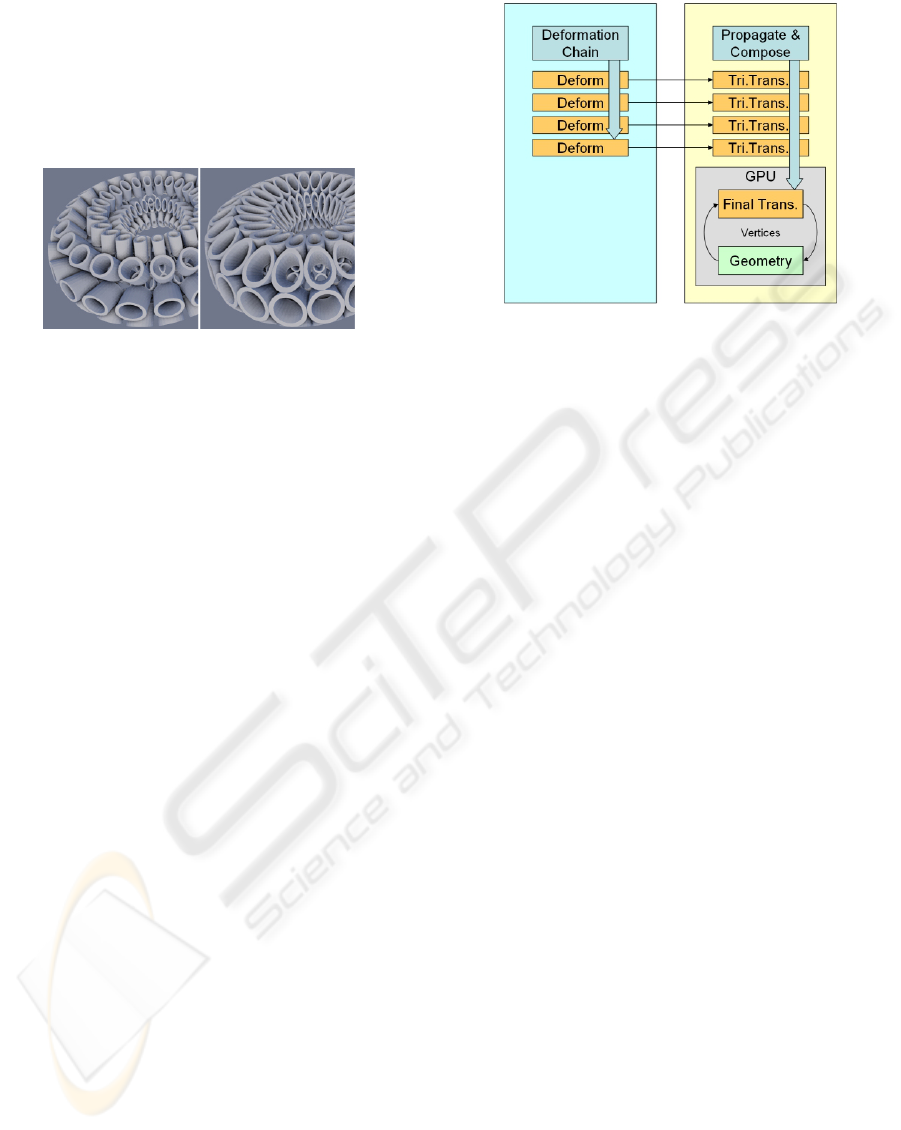
Figure 1: Wrapping a 2D grid of tubes around a torus using
the scene graph’s transformation capabilities only: Using
linear transformations this results in single tubes sticking
out from the torus. With our approach the tubes stay in
contact with each other as they did in the 2D grid.
The used transformation describes a warping of
the 3D space. So any kind of geometrical structure
can be used in conjunction with this transformation
type.
There are two benefits when using this approach.
First, the whole process of a deformation is simpli-
fied, since the scene graph is now able to handle the
deformation itself without the need of external struc-
tures. Second, it allows simple GPU based imple-
mentations, while the handling of the transformation
system itself stays similar to matrix based systems.
Using GPU based transformation, geometry can be
directly deformed during rendering, removing the ne-
cessity to produce and store intermediate deformation
results, see Figure 1.
Our main contribution is an approach for embed-
ding a deformation into a scene graph system by re-
placing the linear 4x4 matrix based transformation of
a scene graph by a more generic trilinear transforma-
tion. Just as linear transformations can be combined
through composition, trilinear transformations can be
composed to allow hierarchical transformations. Ad-
ditionally, we allow assembling several transforma-
tions into a grid for the approximation of arbitrary
non-linear transformations. While the composition of
transformations is performed inside the CPU during
scene graph traversal, all geometric transformations
are computed on the GPU. The composition allows
the GPU to transform the vertices of the geometry in
constant time. This is independent of the depth and
complexity of the transformation hierarchy attached
to it. It is independent of the number of applied defor-
mations over the hierarchy. This is shown in Figure
2.
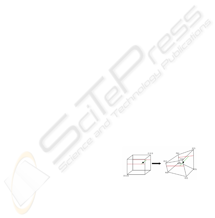
Figure 2: Our approach: Instead of transforming each ge-
ometry vertex in each deformation node, we first approxi-
mate the arbitrary non-linear transformations with our tri-
linear transformation system (left box to right box). During
the scene graph traversal we can now use propagation and
composition of the trilinear transformations. This leads to
one combined transformation used within the vertex trans-
formation stage inside the GPU (right box).
In the next section we review and describe basic
concepts for deformation and scene graphs. Then we
refer to the concept behind trilinear transformations
and we describe our usage of this kind of transfor-
mation. In the implementation section we present the
composition mechanism we use in the transformation
process of geometry and normals. As an application
we present the use of this transformation concept to
handle geometric attachments on the surface of de-
formable geometries. The results section discusses
the abilities and results of the presented approach and
is followed by conclusions and future work.
2 BACKGROUND
2.1 Scene Graphs
Graph structures deal efficiently with hierarchical
relations of objects within scenes. These days,
scene graphs are widely used within graphic applica-
tions. Several systems and application programming
interfaces (APIs) like X3D, Open Inventor (Wang
et al., 1997), OpenGL Performer (Rohlf and Helman,
1994), Java3D (Sowizral et al., 1998), OpenSG (Rein-
ers et al., 2002), Open Scene Graph or the NVIDIA
NVSG provide scene graph based scene management
functionality. Being powerful toolkits, scene manage-
ment and the rendering subsystem are often mixed
and difficult to exchange. To circumvent this, (Ru-
binstein et al., 2009) present a scene graph system
EMBEDDING HIERACHICAL DEFORMATION WITHIN A REALTIME SCENE GRAPH - A Simple Approach for
Embedding GPU-based Realtime Deformations using Trilinear Transformations Embedded in a Scene Graph
247
which is especially designed to fit to different render-
ing methods. This is done by allowing the rendering
process to use a retained mode, to start the rendering
rendering process itself after scene traversal.
2.2 Transformation and Deformation
Candidates for replacing the linear transformation
system of a scene graph are presented in (Gomes
et al., 1998). The authors give a survey over differ-
ent transformation techniques with a focus on warp-
ing and morphing techniques. The presented 2D tech-
niques can be easily extended to 3D. An overview of
existing deformation and animation techniques for 3D
objects is given in (Chen et al., 2005). Physical simu-
lation often uses deformation techniques to apply the
simulation result to a target mesh from a lower reso-
lution control mechanism (Nealen et al., 2005)
An early deformation technique with a focus on
proper handling of the surface normals can be found
in (Barr, 1984). The author presents a group of defor-
mation methods, which additionally allow the com-
putations of proper deformations of the normal. The
nesting of several subsequent deformations is pre-
sented in (Raviv and Elber, 1999) with a focus on
freeform sculpting and modelling. Free Form Defor-
mations (Sederberg and Parry, 1986) allow an intu-
itive way to manipulate objects with deformation us-
ing a control grid. Both methods use local und global
deformations to create level of detail mechanisms for
modifying an object.
Nowadays, deformation topics have moved from
definition and structuring to a more animation and
modelling related view. A number of different ap-
proaches have been proposed to control the deforma-
tion of high polygon models. In (Sumner et al., 2007)
a handle-based approach for manipulating high poly-
gon models is presented. In (Eigensatz and Pauly,
2009) the authors present a different deformation
method based on the manipulation of parts of the
surface’s properties. In (Langer and Seidel, 2008)
the authors propose a deformation method, which ex-
tends the concept of barycentric coordinates in order
to achieve smooth transition between the deformation
elements. In (Botsch et al., 2007) the authors present
a method which is based on elastic coupling of cells to
achieve a smooth transition between user constraints.
In order to generate skin deformation on 3D charac-
ters, user specified chunks are deformed by using a
finite element method to create realistic looking de-
formations of the mesh (Guo and Wong, 2005).
A highly efficient GPU-based approach for cre-
ating wrinkles on textile materials using deformation
was proposed by (Loviscach, 2006). (Popa et al.,
2009) use deformations as a tool to model wrinkles
of garments, which have been captured from video
frames resulting in highly detailed 3D capture result.
2.3 Deformation Embedded Within the
Scene Graph
The presented methods show scene handling and the
use cases for deformation and deformation processes.
As the presented scene graph systems do not take
into account deformation as a low level transforma-
tion process, the aforementioned publications deal-
ing with deformation focus mainly on animation and
modelling aspects. Even though the idea of using a
hierarchy of deformations is not new (Sederberg and
Parry, 1986) (Raviv and Elber, 1999) , the previous
work leave out the possibility of handling hierarchi-
cal deformations in conjunction with object placing
and grouping in 3D scenes for real time applications
on a scene graph level. Our scenario requires an eval-
uation of all transformations of the whole scene per
frame. The nonlinearity of the transformation adds
the functionality to not only group objects, but to ap-
ply these groups to curvatures, greatly increasing the
scene graph’s functionality. In the next section we
show our approach to embed deformation into the
scene graph of a real time rendering system.
3 EMBEDDING TRILINEAR
TRANSFORMATIONS
In this section we describe the trilinear transformation
and how we use it as replacement of the linear trans-
formation within a scene graph.
Figure 3: Trilinear transformation: a point within a unit
cube is transformed by using its three coordinates as coeffi-
cients for a trilinear interpolation between the eight corners
of the cuboid.
3.1 Trilinear Transformations
As described in (Gomes et al., 1998) the trilinear
transformation is an extended version of the bilinear
transformation. It is a function, mapping points of R
3
to R
3
defined by 8 points forming a cuboid, see Figure
3.
GRAPP 2010 - International Conference on Computer Graphics Theory and Applications
248
In contrast to linear transformations each corner
point of the cuboid defines its own coordinate system.
It is created by the three adjacent corner points. A hi-
erarchy of these transformations describes a hierarchy
of local subspaces within a world space. This is com-
pletely different to a linear system, which would de-
scribe a hierarchy of local coordinate systems within
a world coordinate system.
3.2 Vertex Transformations
In general there are two methods to perform the trilin-
ear transformation of a point in space. The first one
uses the coordinates of the cuboid directly to trans-
form vertices, the second one uses a polynomial rep-
resentation allowing fast transformation of many ver-
tices. Additionally, the necessary coefficients allow
a simple test, whether the transformation represents a
parallelpiped or a real cuboid.
The first methods uses the corner points ~p
0
..~p
7
of
the cuboid (see Figure 3) and the transformation T,
defined as
T (x,y, z) =
~p
0
~p
1
~p
2
~p
3
~p
4
~p
5
~p
6
~p
7
T
∗
(1 − x)(1 −y)(1 − z)
x(1 − y)(1 −z)
(1 − x)y(1 −z)
xy(1 − z)
(1 − x)(1 −y)z
x(1 − y)z
(1 − x)yz
xyz
(1)
Here x,y and z are the coordinates of a point to
transform in the range [0..1]. This equation can be
used to directly transform a point. A nice feature of
this approach is the direct usage of the image (cuboid)
of the transformation.
However, with multiplication and sorting by x,y, z
we get a second transformation process using a poly-
nomial representation, where a coefficient matrix C is
created from the corner points of the cuboid:
C =
~p
7
− ~p
6
− ~p
5
+ ~p
4
− ~p
3
+ ~p
2
+ ~p
1
− ~p
0
~p
6
− ~p
4
− ~p
2
+ ~p
0
~p
5
− ~p
4
− ~p
1
+ ~p
0
~p
3
− ~p
2
− ~p
1
+ ~p
0
~p
4
− ~p
0
~p
2
− ~p
0
~p
1
− ~p
0
~p
0
T
(2)
Additionally, a parameter vector~v is built from the
coordinates of the point in space which we want to
transform:
~v = (xyz, yz,xz,xy, z, y, x, 1) (3)
The transformation is now performed by multiply-
ing the vector~v with the matrix C
~
v
0
= C ∗~v (4)
Since matrix C is valid for all points to be trans-
formed, the only computations be to be done are the
construction of ~v and its multiplication with C . We
describe linear transformations as a special case of
the trilinear transformation by keeping the coordinate
systems constant over the volume defined by the
cuboid. This is the case, if the cuboid represents a
parallelpiped. This allows a detection of linear cases
after propagation and composition, see Figure 4.
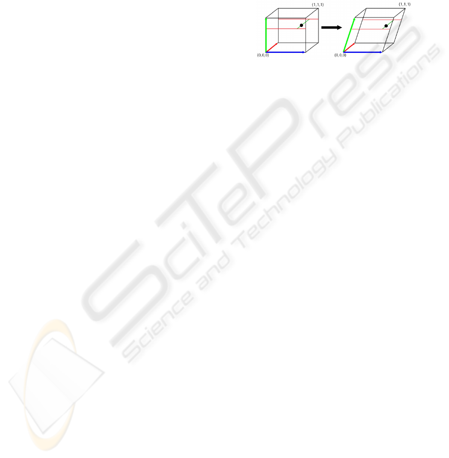
Figure 4: Warping of a unit cube using linear transforma-
tion results in a parallelpiped. This is a special case of a
cuboid.
Taking a closer look at the matrix C and the gen-
eration of coefficients two things are clear. The right
part of C describes a linear 4x3 matrix. It contains
a coordinate system plus an offset. The left side of
C consists of 4 vectors describing the difference be-
tween the parallelpiped defined by the right 4x3 ma-
trix and the intended cuboid. If the transformation de-
scribes a linear transformation this left side of C con-
tains only zeros. This knowledge allows one to test
whether a trilinear transformation is truly a deforma-
tion or just a linear transformation. This is a nice fea-
ture, since this test can be performed after composing
the overall transformation for a geometry directly be-
fore rendering. This test allows one to limit the higher
computational effort necessary for deformation to the
objects really needing deformation without the need
of an extra protocol.
Both methods describe a warping of the whole
space. This allows handling any geometric structure
which can be represented in that space.
3.3 Approximating Arbitrary
Deformations and Composition
Until now we discussed simple trilinear transforma-
tions using only a single cuboid. We will call this
type simple transformation. In order to cope with real
deformations we need a more flexible tool. Fortu-
nately, trilinear transformations have a local charac-
ter and can be attached side by side to form control
grids. These grid structures can be used to approx-
imate complex arbitrary deformations, like it is pro-
posed by (Rezk-Salama et al., 2001). Additional re-
finements of the grid are presented to allow local de-
tails of the deformation. Since our aim is to directly
EMBEDDING HIERACHICAL DEFORMATION WITHIN A REALTIME SCENE GRAPH - A Simple Approach for
Embedding GPU-based Realtime Deformations using Trilinear Transformations Embedded in a Scene Graph
249

use 3D textures of the GPU to store these grids, we de-
cided to use simple uniform grids. Additionally, this
allows us to use trilinear interpolation of the texture
stage to perform the necessary interpolation within a
single cuboid of the grid.
Since we intend to combine assembled transfor-
mations with simple transformations, we have to take
care of the following sampling issue: transforming
the cuboid of a transformation is a sampling process
that will only approximate the original transforma-
tion. If this is another simple trilinear transformation,
this is no problem. A problem arises when an assem-
bled transformation is sampled by one with lower fre-
quency. This will lead to under-sampling. We prevent
this problem by propagating the transformation with
the highest resolution.
4 IMPLEMENTATION
We additionally use bounding boxes to map parts of
the scene to unit cubes. These additional bounding
boxes are defined for each non-linear transformation.
All content of the bounding box is warped into the
cuboid. So in addition to the transformation hierarchy
of the scene graph there is a bounding box hierarchy.
The images of the child transformations have to be
contained inside the parent’s bounding box.
4.1 The Transformation Process
In order to create propagation and composition we use
one transformation (G ) to warp the other (L). In prin-
ciple the composition (C) of two trilinear transforma-
tions C = G ∗ L is computed by transforming the po-
sitions of L’s cuboid grid by the transformation G.
A problem arises from this composition. Our goal
is to compose two trilinear transformations into a new
one. Since composing a child nodes transformation
with the parent nodes transformation does not result
mathematically in an new trilinear transformation.
This happens due to the ability of the trilinear trans-
formation to be able to map lines to curves, which is
always the case, if the image cuboid does not resem-
ble a parallelpiped. To circumvent this problem we
use the child’s transformation cuboid to approximate
the deformation represented by the parent’s cuboid.
Besides from introducing an approximation error this
allows us to get one final composed transformation at
a geometry leaf, which is trilinear, and has to be ap-
plied to the geometry in the vertex processing stage.
Looking at the transformation hierarchy inside a
scene graph we now perform the propagation and
composition process the following way: We propa-
gate the transformation from the world space towards
the local space of the geometry. At each step we have
to transform a more local transformation (L) with the
composition of the more global transformations (G).
The new composed transformation (C ) is now given
by transforming the grid data of the local transforma-
tion L by the old composed transformation G . As a
result the new composition transformation is a trans-
formed copy of L.
As described in section 3.3 this composition of
these transformations resembles a sampling process.
To prevent loss of information we have to choose a
sampling grid for L being equal or finer in structure of
the cells then the grid performing the transformation.
Otherwise we have to handle this problem by increas-
ing the resolution of L’s grid, e.g. by resampling. We
chose the grid size in the following way: Since we use
a bounding box hierachy, L and G having the same
resolution will automatically result in a proper sam-
pling of G since L is smaller in size. Otherwise we
check which transformation uses the highest resolu-
tion and use its grid resolution for computing C . On
the GPU we use interpolated 3D textures to represent
the transformation grids. Since a 3D texture already
has a domain defined in a unit cube, it is only neces-
sary to perform the mapping from the bounding box
to a unit cube in advance. Positions are represented
by float values instead of colours in the texture.
We represent linear transformations only by using
transformations with a grid size of one (one cuboid).
As an optimisation this allows us to check whether
the transformation represents a parallelpiped. If the
final transformation contains a larger grid we always
consider it to handle a non-linear transformation.
Figure 5: For rendering the lighting of the scene it is neces-
sary to handle the deformation of the geometry’s surface
normals. We use two methods. Method 1 (left) simply
transforms the normal with the given transformation. The
resulting normal is not necessarily orthogonal to the surface,
creating a smooth normal transition at the cuboid’s bound-
ary. Method 2 (right) shows the results transforming the
surface’s tangent space. Since the normal is now orthogo-
nal to the surface, visible seams at the cuboid’s border are
noticeable.
GRAPP 2010 - International Conference on Computer Graphics Theory and Applications
250
4.2 Normal Transformations
Since groups of trilinear transformations are of C
0
continuity at their borders, special care have to be
taken when computing the normals for lighting the
contained objects (Rezk-Salama et al., 2001). There
are several methods for computing the normals used
for shading the surfaces (see (Akenine-M
¨
oller et al.,
2008)). For our implementation we have chosen two
computation methods. Using the first method, we
transform the tangent space representation of the nor-
mal. This results in normals orthogonal to the de-
formed surface. With the second method, we trans-
form the normal directly. This results in a smooth
lighting transition between cuboids. In both methods,
transformations have to be performed with respect to
the position of the vertex the normal or tangent space
belongs to. This has to be done due to the position
dependency of the coordinate system in a non paral-
lelpiped cuboid. Both methods are valid and can be
used with this approach (see Figure 5).
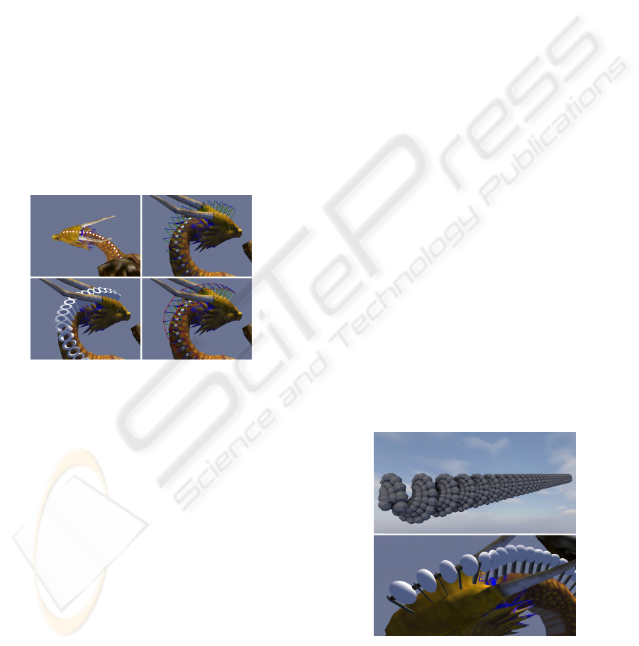
Figure 6: Automated handling of attached geometry in our
method: At first we place a set of anchor points on the
figurine (top left). Barycentric coordinates allow updating
these points if the figurine is deformed or animated. These
points represent local coordinate system (top right). These
coordinate systems are used to create a deformation grid on
the fly (bottom right). The control grid enables the scene
graph to deform the attached geometry (bottom left).
5 APPLICATION EXAMPLE
In order to attach geometry to another surface we need
additional control structures, keeping the deformation
nodes up to date if the surface position changes, see
Figure 6. An attachment consists of a list of anchors
placed on the surface of the target’s geometry, a trans-
formation controlled by the anchors, and the geome-
try object which has to be attached. An anchor is de-
fined by two points, which are registered and mapped
onto a triangle of the basic mesh using barycentric
coordinates. The first point resembles the anchor po-
sition. The second point is used to specify the orien-
tation of the tangent vector. From these two points
and the triangle’s surface normal a coordinate system
is computed. The transformation has to compute a tri-
linear transformation for this list of anchors, depend-
ing on which behaviour the attachment has to have.
An update of the anchors local coordinates system is
performed by barycentric interpolation of the points
of the triangle. This allows the computation of anchor
position and alignment by only using the information
of the geometry, see Figure 6. This concept is inde-
pendent of the animation concept, which is used on
the basic mesh, the anchor is applied to. The coordi-
nate system defined by an anchor resides within the
local space of the geometry. Thus the transformations
dealing with the attachments have to work within the
same space. In our example we use arrays of anchors
to produce a 1D or 2D deformation grids used by the
cuboids.
6 EXPERIMENTAL RESULTS
We have tested the system with several scenes (see
Figure 7). We focused on two aspects of our imple-
mentation. Besides measuring the speed difference
between trilinear transformations and linear transfor-
mations we had to differentiate between the GPU and
the CPU part. In order to measure the vertex through-
put in the GPU we used a high polygon model as de-
formation target. The high polygon count was created
by attaching several highly tesselated spheres to an
animated object. The chain of spheres is deformed
according to the animation of the base mesh. For the
CPU side we created a helix using a large number of
small objects to measure the composition throughput.
Figure 7: The scenes we used for experimentation: For the
CPU tests, we created a helix consisting of many small low
resolution spheres to create a high amount of composition.
For testing the vertex throughput of the GPU, we attached
some high resolution spheres to an animated model. These
spheres are deformed with respect to the animation, using
our method.
EMBEDDING HIERACHICAL DEFORMATION WITHIN A REALTIME SCENE GRAPH - A Simple Approach for
Embedding GPU-based Realtime Deformations using Trilinear Transformations Embedded in a Scene Graph
251
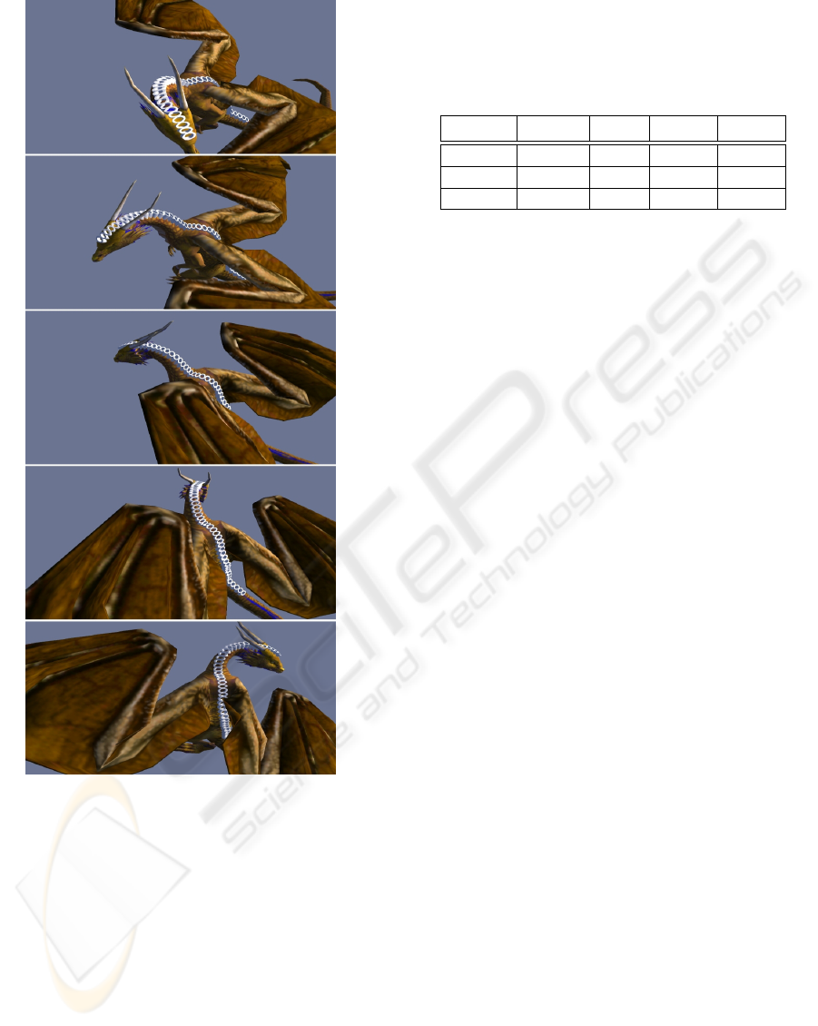
Figure 8: Results: 5 Frames from the vertex animated fig-
urine with a geometric attachment on its back, presenting
the deformation of the attached geometry. The whole pro-
cess is directly managed by the scene graph.
In both tests we compared linear vs. trilinear through-
put in frames per second.
The tests were performed on a system containing
a GForce 8800 and an Intel Core 2 Quad 6600. The
tables show a comparison between the use of trilinear
transformation and the linear transformed scene in
frames per second. Additionally, the number of
objects and triangles are exposed. The software was
implemented in OpenGL. All geometry was stored in
Vertex Buffer Objects (VBO) on the GPU side. The
composition of the trilinear transformations within
the scene graph’s hierarchy is performed on the CPU.
Deformation of the geometry leaf nodes is done per
GPU vertex shader. The trilinear transformation part
of the used shader is roughly two and a half times
more complex compared to the four scalar products
of a linear transformation.
scene objects Tri. FPS/L FPS/T
spheres 185 1.5M 19.5 14.9
helix 4617 164k 16.5 13.3
helix 2566 656k 10.8 8.4
An experiment was performed with a 1.5 mil-
lion triangles object to compare the GPU side of
the transformation stage. Even though the vertex
shader for the trilinear transformation is much more
complex than the linear one, we achieve 75 percent
of the frame rate from the linear vertex shader. The
composition test (CPU) had different results. Using
a large number of low poly models resulted in a
performance decrease to 80 percent (second row).
Increasing the polygon rate by decreasing the amount
of objects (third row) shifts the performance decrease
to 77 percent (third row). Expectedly, this behaviour
results from moving slowly the amount of operations
from composition (CPU) towards transformation
(GPU).
7 CONCLUSIONS AND FUTURE
WORK
We have presented an approach to embed deforma-
tions in a scene graph system by replacing the 4x4
matrix based transformation system by a more generic
one. This extends the usage of transformation nodes
to warping. We achieve this by combining the idea of
trilinear transformation with the hierarchical organi-
sation structure of a scene graph. We support arbitrary
deformations by using an approximation scheme. As
a large benefit we perform all geometric transforma-
tions on the GPU within constant time. The com-
position of the scene graph’s transformations is still
performed inside the CPU. Theoretically, this could
lead to a performance bottlenecks, but only if a huge
multitude of complex transformations have to be com-
posed and send to the GPU. This has not been ob-
served by any of our experiments. As an application
we presented the attachment of arbitrary geometry to
the surface of other deformable or dynamic geometry.
For handling surface normals we have presented two
methods. The first one performs a direct deformation
of the normals. The second method guarantees or-
thogonality to the deformed surface by using the tan-
gent space for normal representation. According to
GRAPP 2010 - International Conference on Computer Graphics Theory and Applications
252
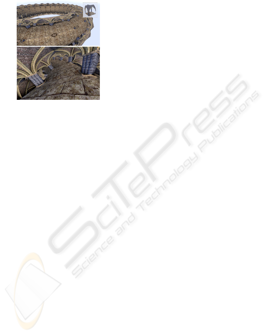
Figure 9: A geometric tile (top right) of a hall mapped on
a torus (top). Inside the 3D model (bottom). The embed-
ded transformation system allows directly the deformation
of the geometric tiles to achieve a seamless (C
0
) joining at
their borders.
(Gomes et al., 1998) the inverse of a trilinear trans-
formation can be computed analogously to the bilin-
ear transformation’s inverse. As we did not need the
inversion for our rendering concept we did not cover
this issue. However, the inverse is often a critical fea-
ture, for example for ray / objects intersections. Addi-
tionally it allows mapping one deformation onto an-
other. Trough an inversion, the integration of structure
based animation concepts (like skeleton based charac-
ter animation) could be mapped into the scene graph
structure. The inversion problem and C
0
continuity
are current drawbacks of the used trilinear deforma-
tion. So a more complex, but invertible and more
continuous transformation scheme could be of higher
benefit in these cases.
REFERENCES
Akenine-M
¨
oller, T., Haines, E., and Hoffman, N. (2008).
Real-Time Rendering 3rd Edition. A. K. Peters, Ltd.,
Natick, MA, USA.
Barr, A. H. (1984). Global and local deformations of solid
primitives. SIGGRAPH Comput. Graph., 18(3):21–
30.
Botsch, M., Pauly, M., Wicke, M., and Gross, M. (2007).
Adaptive space deformations based on rigid cells.
Computer Graphics Forum (Proc. EUROGRAPH-
ICS), 26(3):339–347.
Chen, M., Correa, C., Islam, S., Jones, M. W., y. Shen, P.,
Silver, D., Walton, S. J., and Willis, P. J. (2005). De-
forming and animating discretely sampled object rep-
resentations. Eurographics State of the Art Reports.
Eigensatz, M. and Pauly, M. (2009). Positional, metric,
and curvature control for constraint-based surface de-
formation. Computer Graphics Forum (Proc. EURO-
GRAPHICS), 28(2)(2):551–558.
Gomes, J., Costa, B., Darsa, L., and Velho, L. (1998). Warp-
ing and morphing of graphical objects. Morgan Kauf-
man Publishers, San Francisco, CA.
Guo, Z. and Wong, K. C. (2005). Skinning with deformable
chunks. Computer Graphics Forum (Proc. EURO-
GRAPHICS), 24(3):373–382.
Langer, T. and Seidel, H.-P. (2008). Higher order barycen-
tric coordinates. Computer Graphics Forum (Proc.
EUROGRAPHICS), 27(2)(2):459–466.
Loviscach, J. (2006). Wrinkling coarse meshes on the gpu.
Computer Graphics Forum (Proc. EUROGRAPH-
ICS), 25(3):467–476.
Nealen, A., Mueller, M., Keiser, R., Boxerman, E., and
Carlson, M. (2005). Physically based deformable
models in computer graphics. Eurographics State of
the Art Reports.
Popa, T., Zhou, Q., Bradley, D., Kraevoy, V., Fu, H., Shef-
fer, A., and Heidrich, W. (2009). Wrinkling cap-
tured garments using space-time data-driven defor-
mation. Computer Graphics Forum (Proc. EURO-
GRAPHICS), 28(2)(2):427–435.
Raviv, A. and Elber, G. (1999). Three dimensional freeform
sculpting via zero sets of scalar trivariate functions. In
SMA ’99: Proceedings of the fifth ACM symposium
on Solid modeling and applications, pages 246–257,
New York, NY, USA. ACM.
Reiners, D., Vo, G., and Behr, J. (2002). Opensg: Basic
concepts. In In 1. OpenSG Symposium OpenSG.
Rezk-Salama, C., Scheuering, M., Soza, G., and Greiner,
G. (2001). Fast volumetric deformation on general
purpose hardware. In HWWS ’01: Proceedings of
the ACM SIGGRAPH/EUROGRAPHICS workshop on
Graphics hardware, pages 17–24, New York, NY,
USA. ACM.
Rohlf, J. and Helman, J. (1994). Iris performer: a high
performance multiprocessing toolkit for real-time 3d
graphics. In SIGGRAPH ’94: Proceedings of the 21st
annual conference on Computer graphics and interac-
tive techniques, pages 381–394, New York, NY, USA.
ACM.
Rubinstein, D., Georgiev, I., Schug, B., and Slusallek, P.
(2009). Rtsg: Ray tracing for x3d via a flexible ren-
dering framework. In Proc. of the 14th International
Conference on 3D Web Technology 2009. ACM, New
York, NY, USA.
Sederberg, T. W. and Parry, S. R. (1986). Free-form defor-
mation of solid geometric models. SIGGRAPH Com-
put. Graph., 20(4):151–160.
Sowizral, H., Rushforth, K., and Deering, M. (1998). The
Java 3D API Specification. Addison-Wesley.
Sumner, R. W., Schmid, J., and Pauly, M. (2007). Embed-
ded deformation for shape manipulation. ACM Trans.
Graph., 26(3):80.
Wang, D., Herman, I., and Reynolds, G. J. (1997). The open
inventor toolkit and the premo standard.
EMBEDDING HIERACHICAL DEFORMATION WITHIN A REALTIME SCENE GRAPH - A Simple Approach for
Embedding GPU-based Realtime Deformations using Trilinear Transformations Embedded in a Scene Graph
253
