
FAST DUAL MINIMIZATION OF WEIGHTED TV + L
1
-NORM FOR
SALT AND PEPPER NOISE REMOVAL
S. Jehan-Besson
CNRS, UMR 6158, LIMOS, F-63173, Aubi`ere, France
Jonas Koko
Clermont Universit´e, Universit´e Blaise Pascal, LIMOS, BP 10448, F-63000 Clermont-Ferrand, France
CNRS, UMR 6158, LIMOS, F-63173, Aubi
`
ere, France
Keywords:
Total variation, L
1
norm, Augmented Lagrangian, Fenchel duality, Uzawa methods, Salt and pepper noise
removal.
Abstract: In this paper, the minimization of a weighted total variation regularization term (denoted TV
g
) with L
1
norm
as the data fidelity term is addressed using the Uzawa block relaxation method. Numerical experiments show
the availability of our algorithm for salt and pepper noise removal and its robustness against the choice of the
penalty parameter. This last property is useful to attain the convergence in a reduced number of iterations
leading to efficient numerical schemes. The specific role of the function g in the weighted total variation
term is also investigated and we show that an appropriate choice leads to a significant improvement of the
final denoising results. Using this function, we propose a whole algorithm for salt and pepper noise removal
(UBR-EDGE) that is able to handle high noise levels at a low computational cost.
1 INTRODUCTION
In many image processing problems, a denoising
step is required to remove noise or spurious details
from corrupted pictures. Variational approaches have
gained a wide popularity these years due to the possi-
ble addition of well-chosen regularity terms. Among
the most influential models, we can cite the total vari-
ation minimization framework introduced by Rudin
and Osher (Rudin and Osher, 1994) and Rudin, Osher
and Fatemi (Rudin et al., 1992). In this framework,
given a noisy image f(x), they propose to recover the
original image u(x) by minimizing the total variation
under L
2
data fidelity:
E(u) =
Z
Ω
|∇u(x)|dx+
λ
Z
Ω
(u(x)− f(x))
2
dx, (1.1)
where Ω ⊂ R
2
, is the image domain and
λ
a positive
scale parameter.
Such a minimization allows the recovery of a simple
geometric description of the image u while preserv-
ing boundaries. This framework is then very efficient
when denoising images with flat zones but fails in pre-
serving texture details. It also fails in removing con-
trasted and isolated pixels in images corrupted by a
salt and pepper noise. For such images, the L
1
norm
is better adapted due to its link to median filtering. It
has been used by (Alliney, 1997) and by (Nikolova,
2004; Fu et al., 2006; Bar et al., 2005; Chan et al.,
2004; Chan et al., 2005; Cai et al., 2008; Cai et al.,
2009) for efficient image denoising algorithms.
In this paper, we choose to investigate the rel-
evance of the L
1
norm for salt and pepper noise
removal through the minimization of the following
functional where the regularization term is a weighted
total variation:
E(u) =
Z
Ω
g(x)|∇u(x)|dx+
λ
Z
Ω
|u(x) − f(x)|dx,
(1.2)
where g : Ω → R
+
is a function independent of u.
Such a criterion has been first investigated in (Bres-
son et al., 2007) for shape denoising. The function
g was chosen as an edge indicator function of the in-
put image (e.g., g(x) = 1/(1 + |∇ f|)), which allows
a better preservation of corners and sharp angles for
shape denoising in images corrupted by a Gaussian
noise. In order to use such a criterion for salt and
pepper noise removal, we have to consider two main
issues: the minimization scheme and the choice of an
appropriate function g.
Concerning the first issue, let us remind that the
minimization of the functional (1.2) is not trivial due
68
Jehan-Besson S. and Koko J. (2010).
FAST DUAL MINIMIZATION OF WEIGHTED TV + L1-NORM FOR SALT AND PEPPER NOISE REMOVAL.
In Proceedings of the International Conference on Computer Vision Theory and Applications, pages 68-75
DOI: 10.5220/0002843900680075
Copyright
c
SciTePress

its non differentiability. Recent papers addressed the
minimization of TV + L
1
using various numerical al-
gorithms. For example, standard calculus of varia-
tions and Euler-Lagrange equations can be used to
compute the PDE that will drive the functional u to-
wards a minimum (Bar et al., 2005; Nikolova et al.,
2006; Bresson et al., 2007). This method requires
a smooth approximation of the L
1
norm and a small
time step much be chosen so as to ensure the con-
vergence. This often leads to a large number of it-
erations as mentioned by (Bresson et al., 2007). In
(Chambolle, 2005), the MRF (Markov Random Field)
model is based on the anisotropic separable approxi-
mation (i.e. |∇u| = |D
x
u|+|D
y
u| where D
x
and D
y
are
the horizontal and vertical discrete derivative opera-
tors). This approximation is also used in (Darbon and
Sigelle, 2006a; Darbon and Sigelle, 2006b) where the
authors proposed an efficient graph-cut method. In all
the approaches mentioned above, an approximationor
a smoothing of the L
1
norm is required. Recently, in
(Bresson et al., 2007), following the works of (Chan
et al., 1999; Chambolle, 2004; Aujol and Chambolle,
2005) and more particularly (Aujol et al., 2006), an
elegant fast minimization algorithm based on a dual
formulation is proposed. Thanks to such approaches,
they do not need any approximation or smoothing of
the L
1
norm, they rather take benefit of a convexregu-
larization of the criterion which was first proposed by
(Aujol et al., 2006).
Following this very interesting work, we propose
a new numerical scheme for the minimization of (1.2)
using dual methods. From the criterion (1.2), an aug-
mented Lagrangian formulation (Fortin and Glowin-
ski, 1983) with a penalty term is introduced and
solved using the block relaxation method of Uzawa.
Our algorithm (named UBR) presents the advantage
to be more robust to the choice of the penalty param-
eter than the algorithm proposed by (Bresson et al.,
2007). This parameter can then be chosen so as to de-
crease the number of iterations and consequently the
computational cost.
The second contribution of this paper lies in the
proposition of a novel algorithm for salt and pepper
noise removal. Taking benefit of the weighted total
variation term TV
g
, we propose to study the influ-
ence of well-chosen functions g in order to improve
the denoising results. An efficient algorithm, denoted
UBR-EDGE, is finally proposed for salt and pepper
noise removal. Thanks to the nice properties of UBR
applied to the weighted TV, our algorithm is able to
handle high noise levels at a low computational cost.
Experimental results are provided to attest the avail-
ability of our 3-steps algorithm.
The paper is organized as follows. In Section
2, we present the TV
g
+ L
1
model and the Uzawa
block relaxation method. The role of the weighted TV
for salt and pepper removal and the algorithm UBR-
EDGE are presented in section 3 and illustrated with
some experimental results.
2 EFFICIENT MINIMIZATION
OF TV
g
+ L
1
-NORM
Let Ω be a two-dimensional bounded open domain
of R
d
with Lipschitz boundary. We consider the
following convex energy functional defined, for any
f ∈ L
1
(Ω), any g : Ω → R
+
and any positive param-
eter
λ
:
E(u) =
Z
Ω
g(x)|∇u(x)|dx+
λ
Z
Ω
|u(x) − f(x)|dx
(2.1)
Our aim is the minimization of the energy functional
E, i.e.
min
u∈BV(Ω)
E(u), (2.2)
where BV(Ω) is the subspace of functions u ∈ L
1
(Ω)
of bounded variations.
2.1 An Augmented Lagrangian Method
In order to approximate (2.1) by an augmented La-
grangian and to present our dual method of resolu-
tion, we need to transform the convex minimization
problem into a suitable saddle-point problem by in-
troducing an auxiliary unknown. Let us introduce the
auxiliary unknown p = f − u and rewrite the func-
tional E as
E(u, p) =
Z
Ω
g(x)|∇u(x)|dx+
λ
Z
Ω
|p(x)|dx (2.3)
The unconstrained minimization problem becomes
min
(u,p)∈K
E(u, p). (2.4)
where K = {(u, p) ∈ X × X | u+ p− f = 0 in X},
with the Euclidian space X = R
NxN
equipped with
the L
2
scalar product (u, v). To problem (2.4), we
associate the augmented Lagrangian functional (see
(Koko and Jehan-Besson, 2009) for details) defined
by:
L
r
(u, p;s) = E(u, p) + (s,u+ p− f)
+
r
2
k u+ p− f k
2
, (2.5)
where r > 0 is the penalty parameter and s the La-
grange multiplier. This minimization problem can be
solved using Uzawa block relaxation methods which
FAST DUAL MINIMIZATION OF WEIGHTED TV + L1-NORM FOR SALT AND PEPPER NOISE REMOVAL
69

have been used in nonlinear mechanics for operator
splitting and domain decomposition methods (Fortin
and Glowinski, 1983; Glowinski and Tallec, 1989;
Koko, 2008). Applying the block relaxation method
to the problem defined above, we obtain the following
algorithm:
Minimization process of TV
g
+ L
1
Initialization. p
−1
, s
0
and r > 0 given.
k ≥ 0. Compute successively u
k
, p
k
and s
k
as follows.
Step 1. Find u
k
∈ X such that
L
r
(u
k
, p
k−1
;s
k
) ≤ L
r
(v, p
k−1
;s
k
), ∀v ∈ X.
(2.6)
Step 2. Find p
k
∈ X such that
L
r
(u
k
, p
k
;s
k
) ≤ L
r
(u
k
,q;s
k
), ∀q∈ X. (2.7)
Step 3. Update the Lagrange multiplier
s
k+1
= s
k
+ r(u
k
+ p
k
− f).
The algorithm UBR corresponds to the generic
block relaxation algorithm ALG2 (see, e.g., (Fortin
and Glowinski, 1983; Glowinski and Tallec, 1989)).
Let us now detail the explicit solutions of the different
steps (proofs are given in (Koko and Jehan-Besson,
2009)).
Proposition 2.1 The solution of Step 1 can be given
by:
u
k
= f − p
k−1
+
1
r
(∇· v
∗
− s
k
)
where v
∗
is the solution of:
−∇(∇· v
∗
− ˜p
k−1
) +
1
g
|∇(∇· v
∗
− ˜p
k−1
)|v
∗
= 0.
(2.8)
with ˜p
k−1
= s
k
+ r(p
k−1
− f).
For solving (2.8), we can use the fixed-point proce-
dure of Chambolle (Chambolle, 2004), v
0
= 0 and for
any ℓ ≥ 0
v
ℓ+1
=
v
ℓ
+
τ
∇(∇· v
ℓ
− ˜p
k−1
)
1+ (
τ
/g)|∇(∇· v
ℓ
− ˜p
k−1
)|
, (2.9)
where
τ
> 0.
The solution of Step 2 is detailed in (Koko and Jehan-
Besson, 2009) and reminded below in the whole de-
scription of the algorithm:
Algorithm UBR
Initialization. p
−1
, s
0
and r > 0 given.
Iteration k ≥ 0. Compute successively u
k
, p
k
and s
k
as follows.
Step 1. Set ˜p
k−1
= s
k
+ r(p
k−1
− f) and compute
v
k
with (2.9).
Compute u
k
u
k
= f − p
k−1
+
1
r
(∇· v
k
− s
k
)
Step 2. Compute p
k
p
k
=
0 if |s
k
+ r(u
k
− f)| <
λ
,
f − u
k
−
1
r
h
s
k
−
λ
s
k
+r(u
k
− f)
|s
k
+r(u
k
− f)|
i
if |s
k
+ r(u
k
− f)| ≥
λ
.
Step 3. Update the Lagrange multiplier
s
k+1
= s
k
+ r(u
k
+ p
k
− f).
We iterate until the relative error in u
k
and p
k
be-
comes sufficiently “small”. The convergence of the
algorithm UBR is checked using the following con-
vergence criterion:
q
||u
k
− u
k−1
||
2
2
+ ||p
k
− p
k−1
||
2
2
q
||u
k
||
2
2
+ ||p
k
||
2
2
≤
ε
up
.
The discrete divergence and gradient operators are
given in (Chambolle, 2004).
Note that, each iteration of Algorithm UBR re-
quires the convergence of the Chambolle fixed point
procedure (2.9). The convergence of this loop is
checked using a threshold on the normalized L
2
error
on v
l
.
2.2 Applicability and Robustness
We first test the availability of our UBR algorithm for
salt and pepper noise removal taking classically g = 1
which corresponds to the minimization of TV + L
1
.
The experimental results provided in Figure 1 demon-
strate that noise is correctly removed. Moreover,
the noisy part is captured through the auxiliary un-
known v as displayed in Figure 1.c. With the function
g(x) = 1 and
λ
= 1.5, we find a PSNR of 32.5 dB for
the denoising of a noise of 10%. The parameter
λ
is
a classical smoothing parameter. Choosing a smaller
value leads to a higher blurring of image components.
The influence of this parameter is less sensitive when
using the TV
g
regularization term as demonstrated in
the next section.
In a second step, we want to study the robustness
of the result against the choice of the parameter r. Our
experimental results tend to prove that the algorithm
UBR provides the same denoised images for different
values of r. This is demonstrated by the Figure 2 that
displays the evolution of the PSNR according to the
number of iterations for different parameters r (from
VISAPP 2010 - International Conference on Computer Vision Theory and Applications
70

(a) Noisy image (b) Final u (c) Final v
Figure 1: The images u (PSNR= 32.5dB) and v obtained
after convergence of the algorithm UBR with g(x) = 1 (
λ
=
1.5, r = 20,
ε
up
= 0.0001) for the image “peppers” with a
salt and pepper noise of 10%.
We first test the availability of our UBR algo-
rithm for salt and pepper noise removal taking
1 which corresponds to the min-
. The experimental results
provided in Figure 1 demonstrate that noise is
correctly removed. Moreover, the noisy part is
as dis-
1
5 dB for the
is a classical smoothing parameter. Choosing a
smaller value leads to a higher blurring of image
components. The influence of this parameter is
50 100 150 200
0
5
10
15
20
25
30
35
Iterations
PSNR
PSNR = 32.5dB
r = 10
r = 20
r = 30
r = 100
r = 200
Figure 2: Algorithm UBR (g=1) : Evolution of PSNR
Figure 2: Algorithm UBR (g=1) : Evolution of PSNR dur-
ing iterations (
λ
= 1.5) with r = 10,20,30,100,200 (
ε
up
=
0.0001) for the image “peppers” with a salt and pepper
noise of 10%.
10 to 200). Such a feature then represents an im-
provement of the method proposed in (Bresson et al.,
2007) since the convergence can be obtained without
the need to increase r to infinity. We also report the
number of iterations according to r (Figure 3). In this
case, the optimal value in terms of iterations is ob-
tained for r = 30 with 60 iterations when
λ
= 1.5, and
for r = 10 with 91 iterations when
λ
= 0.5. Choosing
a higher value for r increases the number of iterations
needed to attain the convergence without improving
the final result. We can then choose a small value for
r to obtain a low computational cost without decreas-
ing the quality of the result.
3 SALT AND PEPPER NOISE
REMOVAL
In this section, we first propose to take benefit of the
weighted TV regularization term and of a dedicated
function g in order to increase the quality of the de-
noising results. Our algorithm UBR is then embedded
in a more complete process specified for salt and pep-
per noise removal and named UBR-EDGE.
ob-
tained after convergence of the algorithm UBR with
0001) for the im-
50 100 150 200
0
100
200
300
Iterations
λ
= 0.5
λ
= 1.5
Figure 3: Algorithm UBR (g=1) : Number of iterations for
convergence according to the parameter r with
λ
= 0.5 and
λ
= 1.5 for the image “Peppers” with a salt and pepper
noise of 10%.
3.1 The Role of the Weighted TV
A first improvement of the denoising results can be
obtained using the fact that the dynamic range of the
noise is known. Indeed corrupted pixels take the val-
ues min or max that correspond respectively to the
minimum and maximum values of intensity. In or-
der to embed this information in the function g, we
introduce the following mask function:
m(x) =
α
n
if f(x) = min or max
α
elsewhere.
(3.1)
We choose
α
n
= 1.5 and
α
= 0.5 in order to up-
permost smooth the corrupted pixels. We then take
g(x) = m
σ
(x) where m
σ
(x) = G
σ
∗ m(x) is a slight
regularized version of m (G is a Gaussian of 0-mean
and variance
σ
= 0.5).
Figure 4 displays the resulting images and the cor-
responding values of PSNR while setting g(x) = 1
(first row) and g(x) = m
σ
(x) (second row). Final
images are provided for different values of the reg-
ularization parameter
λ
. For each parameter, we ob-
serve a significant increase of 2 to 4dB in the final
PSNR. The best value of PSNR is 34.9 dB obtained
for
λ
= 1.5. The scale effect of the parameter
λ
is
also less visible due to the fact that we restrict the
regularization term to the extreme values of intensi-
ties corresponding to the corrupted pixels.
Moreover, these first results are obtained at a low
computational cost (from 1.6 seconds for a noise of
10% to 4.3 seconds for a noise of 70% on the image
Peppers (256x256)with a computer of 3GHz and 2Gb
of RAM). This confirms the efficiency of our numer-
ical scheme UBR and attests its availability for the
design of our 3-steps salt and pepper noise removal
algorithm detailed thereafter.
FAST DUAL MINIMIZATION OF WEIGHTED TV + L1-NORM FOR SALT AND PEPPER NOISE REMOVAL
71
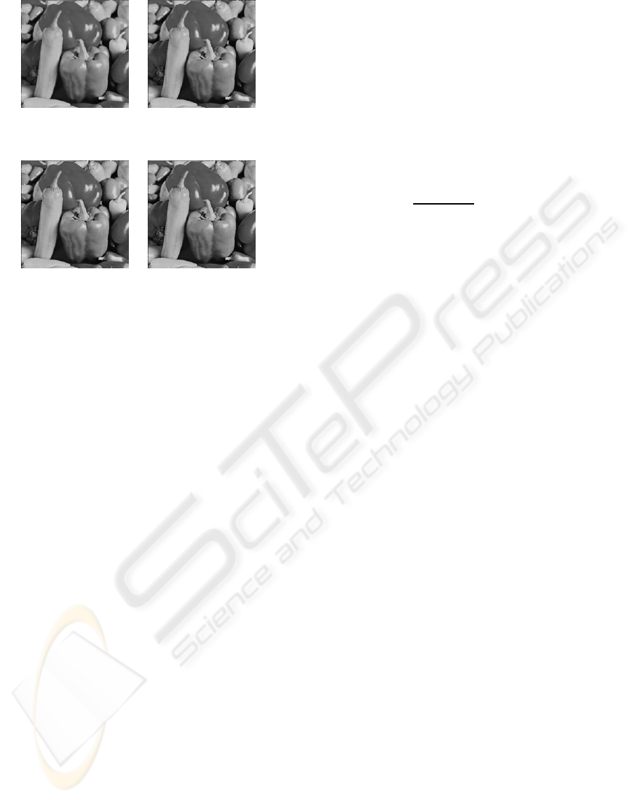
(a)
λ
= 1,g = 1 (b)
λ
= 1.5,g = 1
PSNR= 30.3 dB PSNR= 32.5 dB
(c)
λ
= 1,g = m
σ
(d)
λ
= 1.5,g = m
σ
PSNR= 34.3 dB PSNR= 34.9 dB
Figure 4: Experimental results with the algorithm UBR for
different smoothing values of
λ
(r = 20,
ε
up
= 0.0001) for
the image “peppers” with a salt and pepper noise of 10%.
The first row displays the results obtained with g(x) = 1
while the second row displays the result obtained using
g(x) = m
σ
(x).
3.2 The 3-steps Algorithm UBR-EDGE
The use of the weighted TV provides a significant in-
crease of the quality of the final results. However,
even if the algorithm TV
g
+ L
1
well performs for low
noise values, it gives very smoothed results for higher
noise values. Indeed, in order to remove large noisy
patches, we must decrease the parameter
λ
and so
increase the smoothing of the whole image. In or-
der to circumvent such a problem, we propose both a
pre and post-processing to UBR. As a first step (pre-
processing), we propose to decrease the size of un-
known values (corrupted pixels) using a median filter
(of half-size 1). The pixels that are still corrupted after
this first pass are estimated by computing a mean on
the known 4-connexity neighbours (i.e. we only take
the known values to compute the mean). The aim of
this first pass is to correct the bias introduced by the
extreme intensity values of the noisy pixels (min or
max) in the variational process. This first estimation
is then corrected using the TV
g
+ L
1
algorithm which
is able to smooth differently noisy pixels from uncor-
rupted ones through the g function. This function is
chosen to be m
σ
(x) detailed in section 3.1. The cor-
rupted pixels are computed from the input image but
the function f used in UBR is the result of step 1. At
the end of the process, we apply a very simple edge
smoother also known as EDDI (De Haan and Lod-
der, 2002) usually used in de-interlacing process for
electronic devices. In this efficient edge smoother,
the unknown intensity values are estimated by com-
puting the mean between the two opposite pixels that
share the nearest intensity in a 8-neighborhood. We
apply this simple filtering scheme only on the initial
corrupted pixels.
Algorithm UBR-EDGE
Step 1. Pre-processing
f
1
← median-filter( f,1)
if f
1
(x) = min or f
1
(x) = max then
f
1
(x) =
1
∑
w( f(x
i
))
∑
x
i
∈V
4
(x)
w( f(x
i
)) f(x
i
)
with w( f(x
i
)) = 0 if f(x
i
) = min or max.
Step 2. Algorithm UBR
run UBR with f
1
as the input image and g(x) =
m
σ
(x) defined in (3.1) and computed using the
initial image f.
Step 3. Edge smoother
if f(x) = min or f(x) = max then
u = 0.5∗ (u(x
i
+ l, x
j
+ k) + u(x
i
− l, x
j
− k))
where
(l, k) = argmin
(l,k)∈{−1,1}x{−1,1}
dif f(l, k)
with dif f(l, k) = |u(x
i
+ l, x
j
+ k) − u(x
i
− l, x
j
−
k)|.
Let us remark that the first functional f
1
only acts
as an initial condition of the algorithm UBR in order
to give a first rough estimate for the corrupted pix-
els. The last edge smoother is applied only on the
corrupted pixels as well.
In Figure 5, final results of the different steps of
our process are given for the restoration of the image
“Lena” corrupted by a salt and pepper noise of 70%.
The Figure 5.(b) displays the image obtained after the
pre-processing step (median filter + mean). This im-
age is processed as an input of our algorithm UBR
using g(x) = m
σ
(x) and the result of our UBR algo-
rithm is given in Figure 5.(c). The EDGE smoother
EDDI is then applied which gives the final image of
Figure 5.(d).
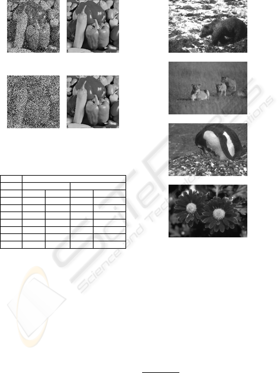
3.3 Experimental Results
Some visual results are provided in Figure 6 for
“Lena” (512x512) and in Figure 7 for “Peppers”
(256x256). Thanks to these visual results and to the
associated PSNR values and computational costs re-
ported for all the noise levels in Table 8, we can con-
clude that our algorithm provides good visual results
VISAPP 2010 - International Conference on Computer Vision Theory and Applications
72
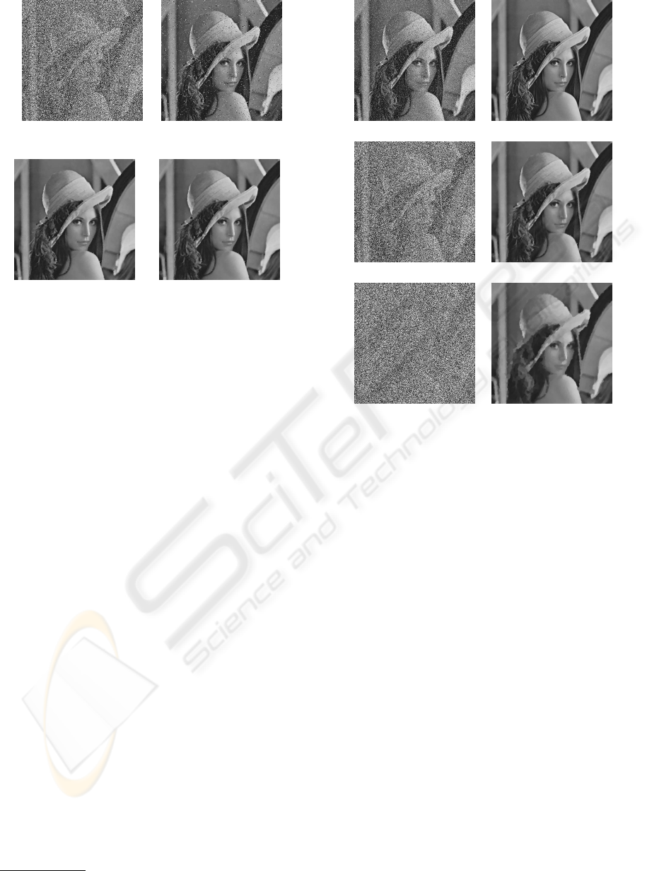
(a) Input image (70%) (b) Step 1
PSNR= 19.6 dB
(c) Step 2: UBR (d) Final : UBR+EDGE
PSNR= 30.1 dB PSNR= 30.6 dB
Figure 5: Salt and pepper noise removal using the algorithm
UBR-EDGE for the image Lena corrupted by a noise of
70%. The result is given for each step of the process. The
image obtained after the pre-processing (median+mean) is
given in (b). This image is used as an input of the algorithm
UBR and the result is given in (c). A last post-processing is
applied to the image which yields to the final result given in
(d).
at a low computational cost. The PSNR values ob-
tained for the image “Lena” can be compared with
the PSNR values reported in (Chan et al., 2004; Chan
et al., 2005) for many different algorithms. Compared
to the values computed in this paper, our algorithm
gives comparable PSNR results to the best algorithm
(i.e. algorithm III) even for a high noise level. For
completeness, we report the values given by (Chan
et al., 2005) for the denoising of Lena (512x512) with
a noise of 70%. With the classical Median filter, the
PSNR is 23.2dB and with an improved switching me-
dian (ISM) filter, the PSNR is 23.4dB. Using the al-
gorithm III proposed in (Chan et al., 2005), the PSNR
is 29.3dB. We find a PSNR of 31.4 dB using our algo-
rithm. For a noise of 90%, they find a PSNR of 25.4
dB while our algorithm gives a PSNR of 26.6 dB. We
also run our algorithm on the input noisy images pro-
vided in the web page of R. Chan
1
. Experimental
results reported in (Koko and Jehan-Besson, 2009)
show that our algorithm gives good quality results
with a PSNR value that is a little smaller than the one
found by the algorithm III (Chan et al., 2004)(with
a difference of less than 1 dB). More precisely, for
the denoising of the first image in Figure 6.a (noise
of 70%), they find a PSNR of 23.07dB while our
1
http://www.math.cuhk.edu.hk/ rchan/paper/impulse/
(a) Noise: 10% (b) PSNR=43.5 dB
(g) Noise: 70% (h) PSNR=31.4 dB
(i) Noise: 90% (j) PSNR=26.6 dB
Figure 6: Salt and pepper noise removal using the algorithm
UBR-EDGE for the image Lena (512x512). The input im-
ages are given with the associated results.
PSNR is 22.2dB. For the image 6.b, they find a PSNR
of 34.16dB while our is 33.3dB. For the image 6.c,
they find a PSNR of 26.78dB while our is 26.0dB. So
their algorithm gives better PSNR for these images
but with a difference of less than 1dB. As far as the
computational cost is concerned, it is difficult to com-
pare the two computational costs since the algorithm
III is programmed using Matlab. However, our al-
gorithm seems to provide a lower computational cost
especially for a high level of noise (see Table 8).
4 CONCLUSIONS
In this paper, our contribution is twofold. First,
we propose a new efficient and robust minimization
scheme for the minimization of a TV
g
+ L
1
criterion
using Uzawa Block Relaxation (UBR) method. We
more particularly study the robustness of the algo-
rithm against the penalty parameter r. Secondly, we
investigate the role of the weighted TV to improve
salt and pepper noise removal and we embed our al-
gorithm in an efficient 3-steps process dedicated to
high noise levels. Our algorithm gives comparable
FAST DUAL MINIMIZATION OF WEIGHTED TV + L1-NORM FOR SALT AND PEPPER NOISE REMOVAL
73
(a) Noise: 30% (b) UBR-EDGE
PSNR=34.5 dB
(c) Noise: 70% (d) UBR-EDGE
PSNR=27.7 dB
Figure 7: Salt and pepper noise removal using the algorithm
UBR-EDGE for “Peppers”. For the result obtained in (b),
λ
=2 and for the result in (d),
λ
= 1.5.
Algorithm UBR-EDGE
Lena (512x512) Peppers (256x256)
Noise PSNR time(s) PSNR time(s)
10 43.4 2.7 40.6 0.4
20 39.7 3.9 37.3 0.7
30 37.1 5.3 34.5 1.1
40 35.3 6.6 32.2 1.4
50 33.9 8.1 30.6 1.7
70 31.4 17.1 27.7 2.3
90 26.6 41.4 23.1 20.1
Figure 8: PSNR according to the salt and pepper noise level
for the image “Peppers” (256x256) and “Lena” (512x512)
using the algorithm UBR-EDGE (r = 200,
ε
up
= 0.0001).
For a noise level between 10% and 50%, we choose the
same value of
λ
= 2. For a noise level of 70%,
λ
= 1.5 and
for 90%,
λ
= 0.7.
PSNR values to one of the best denoising algorithm
available in the literature and at a lower computational
cost. However, we can mention that choosing auto-
matically the value of both the scale parameter and
the penalty parameter in order to obtain the best qual-
ity result and the lower computational cost is an open
question that remains difficult to solve. Our on going
research is directed towards this issue.
(a) PSNR=22.2 dB
(b) PSNR=33.3 dB
(c) PSNR=26.0 dB
(d) PSNR=29.1 dB
Figure 9: Salt and pepper noise removal using the algorithm
UBR-EDGE for different images of the Berkeley database
corrupted with a salt and pepper noise of 70%. For all the
results, we take
λ
= 2.
ACKNOWLEDGEMENTS
The numerical experiments were run in C
++
with the
library Pandore
2
. The salt and pepper noise was gen-
erated with gmic
3
.
REFERENCES
Alliney, S. (1997). A property of the minimum vectors of a
regularizing functional defined by means of the abso-
2
available at http://www.greyc.ensicaen.fr/regis/Pandore/
3
http://gmic.sourceforge.net/
VISAPP 2010 - International Conference on Computer Vision Theory and Applications
74

lute norm. IEEE Transactions on Signal Processing,
45(4):913–917.
Aujol, J.-F. and Chambolle, A. (2005). Dual norms and
image decomposition models. International Journal
of Computer Vision, 63(1):85–104.
Aujol, J.-F., Gilboa, G., Chan, T. F., and Osher, S. (2006).
Structure-texture image decomposition - modeling, al-
gorithms, and parameter selection. International Jour-
nal of Computer Vision, 67(1):111–136.
Bar, L., Sochen, N. A., and Kiryati, N. (2005). Image de-
blurring in the presence of salt-and-pepper noise. In
Kimmel, R., Sochen, N. A., and Weickert, J., editors,
Scale-Space, volume 3459 of Lecture Notes in Com-
puter Science, pages 107–118. Springer.
Bresson, X., Esedoglu, S., Vandergheynst, P., Thiran, J.-P.,
and Osher, S. (2007). Fast global minimization of the
active contour/snake model. Journal of Mathematical
Imaging and Vision, 28:151–167.
Cai, J., Chan, R., and Nikolova, M. (2008). Two-phase
methods for deblurring images corrupted by impulse
plus gaussian noise. Inverse Probl. Imaging, 2:187–
204.
Cai, J., Chan, R., and Nikolova, M. (2009). Fast two-
phase image deblurring under impulse noise. Journal
of Mathematical Imaging and Vision.
Chambolle, A. (2004). An algorithm for total variation min-
imization and applications. Journal of Mathematical
Imaging and Vision, 20(1-2):89–97.
Chambolle, A. (2005). Total variation minimization and a
class of binary MRF models. In Workshop on Energy
Minimization Methods in Computer Vision and Pat-
tern Recognition, pages 136–152.
Chan, R., Ho, C., and M.Nikolova (2005). Salt-and-pepper
noise removal by median-type noise detectors and
detail-preserving regularization. IEEE Transactions
on Image Processing, 14(15):1479–1485.
Chan, R., Hu, C., and Nikolova, M. (2004). An iterative
procedure for removing random-valued impulse noise.
IEEE Signal Processing Letters, pages 921–924.
Chan, T., Golub, G., and P.Mulet (1999). A nonlinear
primal-dual method for total variation-based image
restoration. SIAM Journal of Scientific Computing,
20(6):1964–1977.
Darbon, J. and Sigelle, M. (2006a). Image restoration with
discrete constrained total variation part I: Fast and ex-
act optimization. Journal of Mathematical Imaging
and Vision, 26(3):261–271.
Darbon, J. and Sigelle, M. (2006b). Image restoration with
discrete constrained total variation part II: Levelable
functions, convex priors and non convex cases. Jour-
nal of Mathematical Imaging and Vision, 26(3):277–
291.
De Haan, G. and Lodder, R. (2002). De-interlacing of video
data using motion vectors and edge information. In
International Conference on Consumer Electronics,
pages 70–71.
Fortin, M. and Glowinski, R. (1983). Augmented La-
grangian Methods: Application to the Numerical So-
lution of Boundary-Value Problems. North-Holland,
Amsterdam.
Fu, H., Ng, M. K., Nikolova, M., and Barlow, J. L. (2006).
Efficient minimization methods of mixed l2-l1 and l1-
l1 norms for image restoration. SIAM J. Scientific
Computing, 27(6):1881–1902.
Glowinski, R. and Tallec, P. L. (1989). Augmented La-
grangian and Operator-splitting Methods in Nonlinear
Mechanics. SIAM, Philadelphia.
Koko, J. (2008). Uzawa block relaxation domain decompo-
sition method for the two-body contact problem with
Tresca friction. Comput. Methods. Appl. Mech. En-
grg., 198:420–431.
Koko, J. and Jehan-Besson, S. (2009). An augmented
lagrangian method for TVg+L1-norm minimization.
Technical Report RR-09-07, Laboratory LIMOS.
Nikolova, M. (2004). A variational approach to remove
outliers and impulse noise. Journal of Mathematical
Imaging and Vision, 20(1-2):99–120.
Nikolova, M., Esedoglu, S., and Chan, T. F. (2006). Al-
gorithms for finding global minimizers of image seg-
mentation and denoising models. SIAM Journal of Ap-
plied Mathematics, 66(5):1632–1648.
Rudin, L. and Osher, S. (1994). Total variation based im-
age restoration with free local constraints. In ICIP,
volume 1, pages 31–35, Austin, Texas.
Rudin, L., Osher, S., and Fatemi, E. (1992). Nonlinear total
variation based noise removal algorithms. Physica D.,
60:259–268.
FAST DUAL MINIMIZATION OF WEIGHTED TV + L1-NORM FOR SALT AND PEPPER NOISE REMOVAL
75
