INTRODUCING SHAPE CONSTRAINT VIA LEGENDRE
MOMENTS IN A VARIATIONAL FRAMEWORK FOR CARDIAC
SEGMENTATION ON NON-CONTRAST CT IMAGES
Julien Wojak, Elsa D. Angelini and Isabelle Bloch
Institut Telecom, T´el´ecom ParisTech, CNRS LTCI, 75013 Paris, France
Keywords:
Segmentation, Medical imaging, Shape constraint.
Abstract:
In thoracic radiotherapy, some organs should be considered with care and protected from undesirable radiation.
Among these organs, the heart is one of the most critical to protect. Its segmentation from routine CT scans
provides valuable information to assess its position and shape. In this paper, we present a novel variational
segmentation method for extracting the heart on non-contrast CT images. To handle the low image contrast
around the cardiac borders, we propose to integrate shape constraints using Legendre moments and adding
an energy term in the functional to be optimized. Results for whole heart segmentation in non-contrast CT
images are presented and comparisons are performed with manual segmentations.
1 INTRODUCTION
In thoracic radiotherapy, some organs should be con-
sidered with care and protected from undesirable ra-
diation. Among these organs, the heart is one of the
most critical in this context. It is therefore useful
to have a good knowledge of the heart position and
shape, for applications such as dose estimation and
therapy planning. This information can be provided
by image segmentation. Routine examinations rely on
non-contrast CT scans, in which the heart is often dif-
ficult to distinguish from surroundingstructures based
on only grey level information. Manual segmentation
is tedious and prone to inter-observer variability, thus
calling for automated methods, we which address in
this paper.
Among the existing approaches, in (Ecabert et al.,
2008) a multi-chamber (i.e. complete heart) mesh
model is deformed to segment the heart on high con-
trast and high resolution CT images. Unfortunately,
this method does not apply to non-contrast CT. In
(Moreno et al., 2008), the segmentation is constrained
using fuzzy representations of anatomical knowledge
about the position of the heart in the thorax and with
respect to the lungs. This leads to a good robustness
but to an average similarity index when compared to
manual segmentation of 0.74, which might be too lim-
ited for radiotherapy applications.
In this paper, we propose to integrate shape con-
straints into a variationalmethod,followingtheidea of
(Foulonneau et al., 2006), and based on the model of
(Mory and Ardon, 2007). Shape information is rep-
resented using Legendre moments and integrated as
an additional energy term in the functional to be opti-
mized. Results for whole heart segmentation on non-
contrast CT images are presented and evaluated.
50 100 150 200
20
40
60
80
100
120
140
160
50 100 150 200
5
10
15
20
25
30
35
40
45
50
55
Figure 1: Non-contrast CT thoracic images with manual
heart segmentations.
2 VARIATIONAL
SEGMENTATION BASED ON
GRAY LEVEL INTENSITY
In (Mory and Ardon, 2007), the authors introduced
a fuzzy region competition framework to segment
an image I into two classes (background and fore-
ground) based on the minimization of the following
functional:
209
Wojak J., D. Angelini E. and Bloch I. (2010).
INTRODUCING SHAPE CONSTRAINT VIA LEGENDRE MOMENTS IN A VARIATIONAL FRAMEWORK FOR CARDIAC SEGMENTATION ON
NON-CONTRAST CT IMAGES.
In Proceedings of the International Conference on Computer Vision Theory and Applications, pages 209-214
DOI: 10.5220/0002844502090214
Copyright
c
 SciTePress

min
u∈BV
[0,1]
(Ω)
E
TV
g
(u(x),α
i
) = min
u∈BV
[0,1]
(Ω)
Z
Ω
g|∇u|dΩ
| {z }
regularity
+ τ

Z
Ω
u(x)r
α
i
(x)dΩ

| {z }
fidelity to the data
(1)
where u is a membership function in BV
[0,1]
(Ω) (the
space of functions of bounded variations), g is a
weighting function of the regularization term in or-
der to relax the regularization near important con-
tours (for example g =
1
1+|∇
˜
I|
with
˜
I a smooth version
of I), and x denotes the coordinates triplet (x,y,z).
The function r
α
i
(x) (α
i
is a set of parameters) could
have different expressions such as the well known
Chan and Vese region competition term r
c
1
,c
2
(x) =
(I −c
1
)
2
−(I −c
2
)
2
where c
1
and c
2
are the mean in-
tensity in each region (Chan and Vese, 2001), or Para-
gios and Deriche geodesic active region term r(x) =
ln
P(I|α
1
)
P(I|α
2
)
(Paragios and Deriche, 1999). The formula-
tion in Equation 1 leads to several interesting proper-
ties:
• using a membership function u instead of a classi-
cal indicator function as in (Chan and Vese, 2001)
leads to a greater stability of the segmentation pro-
cess and to a better control of the regularity of the
final contours;
• as the space of solutions is the BV space, the
membership function u converges toward an indi-
cator function, and therefore a simple threshold-
ing at the end of the minimization process pro-
vides the final segmentation;
• as the regularization term is convex, the final re-
sult is not sensitive to the initialization.
In this work, we use the region competition ap-
proach, with the same formulation as in Equation 1,
leading to a fast and flexible segmentation tool to ex-
tract the lung cavities and internal blood vessels as
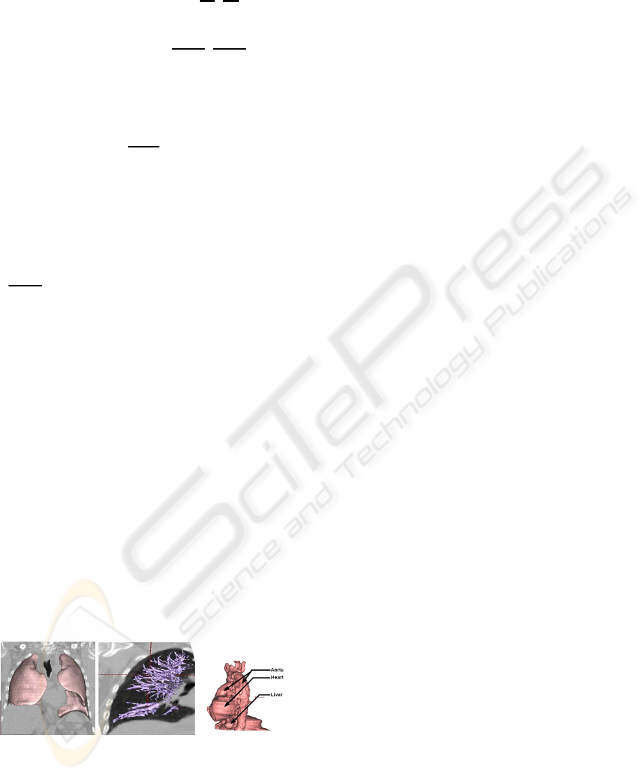
illustrated in Figure 2(a-b).
(a) (b) (c)
Figure 2: Segmentation using the region competition for-
mulation: (a-b) lungs and lung vessels (c) the heart is not
well separated from the liver and the aorta.
However, since this approach only relies on in-
tensity discrimination into two classes (or phases),
it cannot segment different structures having similar
gray level characteristics. An example in 2(c) illus-
trates the difficulty of separating the heart from adja-
cent structures such as the major blood vessels and the
liver, on non-contrast CT data. In order to overcome
such limitations, we propose to constrain the segmen-
tation using shape information.
3 SHAPE CONSTRAINT
Several methods have been proposed to constrain
shapes in a segmentation functional. In (Gastaud
et al., 2004), a distance between a reference and the
observed shapes is used. In (Leventon et al., 2000),
a PCA analysis is performed on the level sets func-
tions of training segmentations. A review of shape
constraints for level sets segmentation methods can
be found in (Cremers et al., 2007). For the fore-
seen applications for thoracic radiotherapy, we have
to achieve a compromise between the constraint on
the shape characterization and the flexibility of the
representation to cope with inter-patient variability
(patient positioning, heart size,... ). In this context it is
not relevant to compute directly a difference between
a reference shape and the current shape segmentation.
We prefer to control an indirect match by comparing
our segmentation with a generic shape model repre-
sentation that does constrain natural anatomic vari-
ability, and is not sensitive to translation and scale
variability. Such characteristics can be provided by
well-chosen shape moments. For example in (Rose
et al., 2009), Tchebichev moments are used to con-
strain a region growing algorithm, and Foulonneau et
al. (Foulonneau et al., 2006) used Legendre moments
as shape descriptors in an active contour segmentation
framework.Our approach follows a similar scheme as
in this last work.
3.1 Legendre Moments
In (Teague, 1980), Teague introduced moments for
image analysis. He proposes to use Legendre poly-
nomials or Zernike polynomials as kernel functions.
This is motivated by the orthogonality property of
both types of polynomials, which guarantees the non-
redundancy of the description of an image or a shape.
The existence of efficient methods to easily and fastly
compute Legendre moments has guided our prefer-
ence for these moments over Zernike ones. Legen-
dre moments are more sensitive to noise than Zernike
moments, but in our framework we manipulate de-
scriptors only on clean binary masks or membership
functions defined on [0, 1], in a framework of fuzzy
VISAPP 2010 - International Conference on Computer Vision Theory and Applications
210

region competition. Therefore this limitation is not a
drawback for the proposed approach.
Legendre moments are defined by the projection
of a function on a polynomial basis. Let I : [−1, 1]
3
→
R be the image representation. The moment of I of
order p+ q+ r is defined as:
λ
pqr
= C
pqr
Z
[−1,1]
3
P
p
(x)P
q
(y)P
r
(z)I(x, y,z)dxdydz
(2)
where C
pqr
=
(2p+1)(2q+1)(2r+1)
8
and P
p
,P
q
,P
r
are Leg-
endre polynomials, defined by the following two or-
der recursive relation:
P
p+1
(x) =
2p + 1
p+ 1
xP
p
(x) −
p
p+ 1
P
p−1
(x) (3)
(p > 1, P
0
(x) = 1 and P
1
(x) = x).
Legendre polynomials form an orthogonal basis,
with:
2p + 1
2
Z
1
−1
P
p
(x)P
q
(x)dx =

0 if p 6= q
1 if p = q
(4)
Working with a finite number of moments, an es-
timate
ˆ
I of I is given by:
ˆ
I(x,y,z) =
L
∑
p=0
p
∑
q=0
q
∑
r=0
λ
p−q,q−r,r
P
p−q
(x)P
q−r
(y)P
r
(z)
(5)
where L is the maximum order for which Legendre
moments are computed.
The computation can be performed with the fast
and exact Hosny method (Hosny, 2007). First, the
spatial image domain is embedded in the cube U =
[−1,1]
3
. Assuming that the image has X ×Y ×Z vox-
els, the centers of voxels are then given by the coordi-
nates (x
i
,y
j
,z
k
) such that
x
i
= −1+ (i−1/2)∆x i = 1···X and ∆x =
2
X
y
j
= −1 + ( j −1/2)∆y j = 1···Y and ∆y =
2
Y
z
k
= −1+ (k −1/2)∆z k = 1···Z and ∆z =
2
Z
(6)
Voxels on wich the image intensity is constant
are then defined as intervals [U
i
,U
i+1
] ×[V
j
,V
j+1
] ×
[W
k
,W
k+1
] with
U
i
= x
i
−∆
x
/2 U
i+1
= x
i
+ ∆
x
/2
V
j
= y
j
−∆
y
/2 V
j+1
= y
j
+ ∆
y
/2
W
k
= z
k
−∆
z
/2 W
k+1
= z
k
+ ∆
z
/2
(7)
The moment expression computed on the whole
image can then be rewritten as:
λ
p,q,r
= C
p,q,r
L
∑
i=1
M
∑
j=1
N
∑
k=1
I(x
i
,y
j
,z
k
)
Z
U
i+1
U
i
Z
V
j+1
V
j
Z
W
k+1
W
k
P
p
(x)P
q
(y)P
r
(z)dxdydz
(8)
Moreover thanks to the following recursive prim-
itive property of the Legendre polynomes
Z
x
cst
P
p
(y)dy =
P
p+1
(x) −P
p−1
(x)
2p+ 1
, (9)
Legendre moments can be written as:
λ
pqr
=
L
∑
i=1
M
∑
j=1
N
∑
k=1
I
p
(x
i
)I
q
(y
j
)I
r
(z
k
)I(x
i
,y
j
,z
k
) (10)
where I
p
(x
i
) =
2p+1
2p+2
[xP
p
(x) −P
p−1
(x)]
U
i
+1
U
i
and sim-
ilar expressions for I
q
and I
r
. The kernel I
p
I
q
I
r
is in-
dependent of the image intensity and can therefore be
precomputed. Moreover the separability property al-
lows us to compute the 3D moments using three 1D
steps.
To guarantee scale and translation invariances,
Legendre moments must be reformulated in the fol-
lowing way:
Λ
pqr
= C
pqr
Z
[−1,1]
3
P
p
(
x−x
0
A
)P
q
(
y−y0
A
)P
r
(
z−z
0
A
)I(x, y, z)dxdydz (11)
where (x
0
,y
0
,z
0
) are the coordinates of the center of
inertia of I and A is the volume of the shape.
3.2 Discriminating Volumes by a Finite
Number of Legendre Moments
Two similar shapes have the same set of Legendre
moments and two different shapes have two different
sets of Legendre moments. However, since we work
with scale and translation invariant moments, the set
{λ
0,0,0
,λ
0,0,1
,λ
0,1,0
,λ
1,0,0
} is the same for each shape
and should not be used for discriminating between
shapes. In order to illustrate the discriminative power
of the moments, we consider four classes of shapes:
class 1: heart alone, class 2: heart and aorta together,
class 3: heart and liver together, class 4: heart and
liver and aorta together.
Norm 2 Error. To highlight differences between
Legendre moments of the four classes of shapes, we
compute the square ℓ
2
norm between two shapes as
||λ
shape
1
−λ
shape
2
||
2
2
where λ
shape
i
is a vector storing
successive Legendre moments of a shape. Comparing
the measures for a finite number of moments from a
mask of a reference heart and objects for the other
classes we obtain the following results (Table 1):
Errors at order 5 are inferior to those at order
15. This is due to the fact that small order moments
represent low frequency shape information. The gap
between moment differneces between hearts and be-
tween hearts and other structures is more important
for order 5 (factor 5) than for order 15 (factor 2). It is
due to the fact that at order 5, the difference between
INTRODUCING SHAPE CONSTRAINT VIA LEGENDRE MOMENTS IN A VARIATIONAL FRAMEWORK FOR
CARDIAC SEGMENTATION ON NON-CONTRAST CT IMAGES
211

Table 1: ℓ
2
norm of the difference between sets of Legendre
moments between a reference heart shape and 13 maks of
others hearts, 4 masks of hearts and liver, 4 masks of hearts
and aorta, 4 masks of hearts and aorta and liver.
mean min max
P
P
P
P
P
P
ref vs
order
5 15 5 15 5 15
other hearts 0.17 1.21 0.13 1.09 0.26 1.52
heart and liver 0.56 2.40 0.52 2.26 0.58 2.56
heart and aorta 0.61 2.38 0.44 2.13 0.69 2.50
heart and aorta
0.53 2.38 0.45 2.19 0.62 2.60
and liver
(a) (b) (c) (d) (e)
Figure 3: Examples of mask of: (a) reference heart, (b-c)
two other hearts, (d) heart and aorta, (e) heart and liver.
shapes of different classes is sufficiently important to
discriminate between them, and in the same class dif-
ferences of the shape are too small to well discrimi-
nate between them.
In the following experiment we compare moments at
a maximum order 10 in order to well differentiate
shapes and to take advantage of the global represen-
tation of a shape by its moments.
PCA Analysis. In this section, we study the capa-
bility of Legendre moments to efficiently discrimi-
nate between correctly segmented hearts and erro-
neous segmentations, by considering again the four
classes of shapes. Inspired by (Poupon et al., 1998),
we performed a PCA analysis on a matrix in which
each raw is an observation, i.e. a segmentation re-
sult, and each column corresponds to an ordered list
of Legendre moments. The PCA analysis shows that
the first three modes represent 90% of the variance.
As illustrated in Figure 4, the moments also discrim-
inate efficiently the different types of shapes. Indeed
samples from the heart alone are well grouped in the
plane of the first two modes and are well separated
from the other types of shapes.
3.3 Introducing Shape Constraint in the
Functional
We propose to introduce an additional term in the seg-
mentation functional to be optimized through a com-
parison between moments of a reference shape and
moments of the current segmented shape, as follows:
Heart
Heart and Liver
Heart and Liver
Heart and Aorta
Heart and Liver and Aorta
first mode
second mode
Figure 4: PCA on Legendre moments. Result on the first
two principal axes, “+” heart alone, “o” heart and liver, “*”
heart and aorta, “x” heart and liver and aorta.
min
u∈BV([0,1])
Z
Ω
g|∇u|dΩ+ τ
Z
Ω
r(x)udΩ
+
γ
2
||λ
ref
−λ
cur
(u)||
2
2
(12)
This formulation is quite similar to the one de-
scribed in (Foulonneau et al., 2006). However, using
a membership function u instead of a level set func-
tion leads to a more stable algorithm. Another differ-
ence concerns the order of the used moments. Since
one of the main objectives of the work by (Foulon-
neau et al., 2006) was to provide an algorithm ro-
bust to occlusions, a hard constraint on the shape was
needed and high order moments were computed. In
our framework, the goal is to capture global features
of the shape and allow a small variability between
them. Therefore only quite small order moments are
needed.
Minimization. We perform the minimization of the
functional (12) by a gradient descent method.
To insure that u ∈ BV
[0,1]
(Ω) in (1) we rewrite it in the
same manner as in (Chan et al., 2005) :
min
u
E
TV
g
(u(x)) = min
u
Z
Ω
g|∇u|dΩ+ τ

Z
Ω
u(x)r(x)dΩ

+
Z
Ω
αν
ε
(u)dΩ +
γ
2
||λ
ref
−λ
cur
(u)||
2
2
(13)
where ν
ε
is a regularized approximation of the pe-
nality function ν(a) = max{0, 2|a −1/2|− 1} with
α > ||r(x) + ||||λ
ref
−λ
cur
(u)||
2
2
||
∞
and we obtain the following iterative scheme:
u
(n+1)
(x) = u
n
(x) + dt

div(g
∇u(x)
|∇u(x)|
) −τr(x) −αν
′
ε
(u)
−γ
∑
p,q,r

(λ
ref
p,q,r
−λ
cur
p,q,r
(u))P
p
(x)P
q
(y)P
r
(z)
i
Choise of r. Let us arbitrarily define the heart region
as the foreground region, (i.e. the region in which we
would like to obtain u(x) = 1) and the rest of the re-
gion of interest as the background region (i.e. the re-
gion in which we would like to obtain u(x) = 0).
Histograms of the foreground and the background
VISAPP 2010 - International Conference on Computer Vision Theory and Applications
212

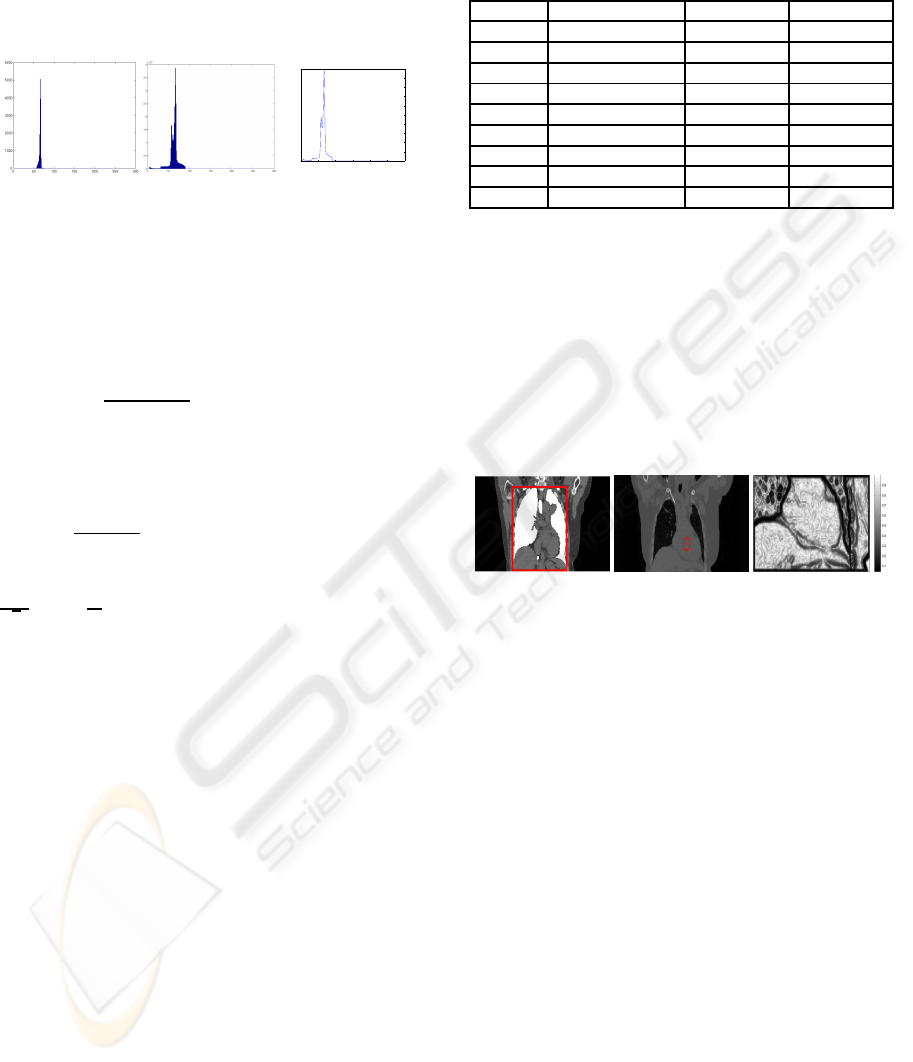
intensities,obtained from manual segmentations, are
shown in Figure 5. It shows that intensities values
are quite similar in the background and in the fore-
ground. However, the intensity is very homogeneous
in the heart and presents two peaks in the background.
0 50 100 150 200 250 300
0
0.01
0.02
0.03
0.04
0.05
0.06
0.07
0.08
0.09
0.1
Figure 5: Histograms of foreground (left) and background
(middle) intensities. Right: background intensity probabil-
ity density estimation using Parzen window.
We use this difference to construct the following
relevant data fidelity term r(x):
r(x) = (I −c
1
)
2
−(max((I −c
1
)
2
))(
Z
B
(p(b) −K(I −b))
2
db (14)
where c
1
=
R
Ω
I(x)u(x)dx
R
Ω
u(x)dx
is the empirical estimation
mean of the heart intensity, B is the interval of the im-
age intensities, p is the Parzen estimation of the prob-
ability density function of the intensity of the back-
ground, expressed as:
p(b) =
1
||1−u||
1
Z
Ω
(1−u(x))K((I(x) −b)/σ)dx (15)
where K is a Gaussian window (K(a) =
1
√
2π
exp(−
a
2
2
)) and σ is chosen sufficiently small to
distinguish the two modes in the background area.
Choice of τ and γ. CT images are calibrated, whith
known tissue intensity values (for examples compact
bones are known to be around 1000 Hounsfield units
(HU)). This intensity inter-images stability calibra-
tion allows us to pre-set the weight of each term in
the functional in order to insure a good balance be-
tween them. The regularization term, computed on
manual segmentations, is of the order of 10
6
(it corre-
sponds to the surface of the whole heart weighted by
g). The data fidelity term is close to zero. The shape
constraint term at order 10 falls within the range of
values [1, 2]. Finally, by dividing g by 10
6
a good
balance between all terms in the functional (12) is ob-
tained for τ and γ in ]0, 10[. We performed several
experiments for different parameters and finally we
fixed τ = 1.4 and γ = 0.8 for all tests summarized in
Table 2.
Table 2: Quantitative results: comparison between auto-
matic and manual segmentations. The numbers in paren-
theses are results obtained by (Moreno et al., 2008).
similarity index sensitivity specificity
Heart 1 0.82 (0.77) 0.96 (0.96) 0.74 (0.64)
Heart 2 0.81 (0.70) 0.89 (0.90) 0.78 (0.58)
Heart 3 0.80 (0.75) 0.94 (0.78) 0.70 (0.72)
Heart 4 0.84 (0.74) 0.76 (0.62) 0.97 (0.92)
Heart 5 0.77 (0.84) 0.81 (0.83) 0.72 (0.84)
Heart 6 0.81 (0.80) 0.93 (0.91) 0.71 (0.71)
Heart 7 0.78 (0.71) 0.84 (0.88) 0.73 (0.60)
Heart 8 0.80 (0.67) 0.92 (0.71) 0.80 (0.62)
Heart 9 0.75 (0.64) 0.83 (0.60) 0.73 (0.70)
4 HEART SEGMENTATION
Masking a Region of Interest and Initializing.
From a pre-segmentation of the lungs, a region of in-
terest (ROI) around the heart is built as the bounding
box of lungs elongated at the bottom to insure that the
heart is completely inside. A mask of the lungs and
the trachea is removed from the ROI.
(a) (b) (c)
Figure 6: Preprocessing. (a) Heart ROI with lungs and
trachea masked out. (b) Example of an initialization of
the hear segmentation. (c) Gradient weighting function g
around the heart.
Moreover tissues at the right of the left lung and
at the left of the right lung are removed. This is illus-
trated in Figure 6.
The initialization is performed semi-automatically. A
point C approximatively at the center of the heart is
marked and the initial value of u(x) is defined by
u(x) = 1 if x is both inside a sphere centered at C
with 4 cm diameter and inside the region of interest,
and u(x) = 0 otherwise.
Tests and Results. Tests on 9 non contrast CT scan
have been performed. For each one, the result of
the segmentation was compared with a manual delin-
eation done by an expert. Similarity, sensitivity and
specificity indices are computed and reported in Table
2. We also compared our results with those obtained
by the method of Moreno (Moreno et al., 2008). We
globally obtain better results than those obtained by
Moreno et al. Differences between the results of the
two methods are illustrated in Figures 7(b) and 8. Ex-
INTRODUCING SHAPE CONSTRAINT VIA LEGENDRE MOMENTS IN A VARIATIONAL FRAMEWORK FOR
CARDIAC SEGMENTATION ON NON-CONTRAST CT IMAGES
213

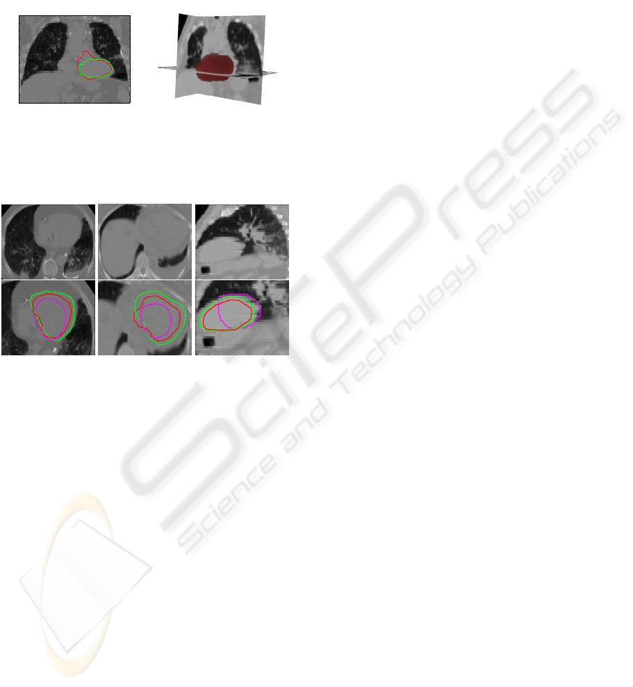
cept for the heart 4 (Figure 8 column 2), the speci-
ficity index is generally higher than the sensitivity. It
means that our automatic segmentation often provides
a larger region than the manual one (it is mainly due
to the fact that a small part of the aorta is often in-
cluded in the segmentation of the heart, as illustrated
in Figure 7(a).
50 100 150 200
5
10
15
20
25
30
35
40
45
50
55
(a) (b)
Figure 7: (a) Automatic segmentation (in red) includes
small part of the aorta (green: manual segmentation). (b)
A 3D view of a whole heart segmentation.
Figure 8: Examples of segmentation results. First row:
original image, second row: image superimposed with seg-
mentations (green expert segmentation, magenta Moreno et
al segmentation, red our automatic segmentation).
5 CONCLUSIONS
We have adapted a fuzzy region competion frame-
work for the segmentation of the heart in non-contrast
CT images by adding a shape constraint. Shape infor-
mations was encoded with Legendre moments. Since
we work with CT images (which are calibrated), we
use hard a priori on the image intensity. The ini-
tialization is performed semi-automatically using a
spherical approximation of the heart. Several tests
on clincal cases provide satisfying results. In par-
ticular, the shape constraint allows us to achieve a
good separation between the heart and surrounding
organs (liver, aorta), improving the initial fuzzy re-
gion competition model. When compared to another
method (Moreno et al., 2008) using structural knowl-
edge (but no shape information) the results are also
improved. This framework could be extended in a se-
quential way to segment other organs in the thorax
like the aorta.
ACKNOWLEDGEMENTS
This work was partially funded by the Medicen Pˆole
de Comp´etitivit´e within the Miniara project.
REFERENCES
Chan, T. F., Esedoglu, S., and Nikolova, M. (2005). Finding
the global minimum for binary image restoration. In
ICIP, pages I: 121–124.
Chan, T. F. and Vese, L. A. (2001). Active contours with-
out edges. IEEE Trans. Image Processing, 10(2):266–
277.
Cremers, D., Rousson, M., and Deriche, R. (2007). A re-
view of statistical approaches to level set segmenta-
tion: Integrating color, texture, motion and shape. In-
ternational Journal of Computer Vision, 72(2):195–
215.
Ecabert, O., Peters, J., and etal (2008). Automatic model-
based segmentation of the heart in CT images. IEEE
Trans. Medical Imaging, 27(9):1189–1201.
Foulonneau, A., Charbonnier, P., and Heitz, F. (2006).
Affine-invariant geometric shape priors for region-
based active contours. IEEE Trans. Pattern Analysis
and Machine Intelligence, 28(8):1352–1357.
Gastaud, M., Barlaud, M., and Aubert, G. (2004). Combin-
ing shape prior and statistical features for active con-
tour segmentation. IEEE Trans. Circuits and Systems
for Video Technology, 14(5):726–734.
Hosny, K. M. (2007). Exact Legendre moment compu-
tation for gray level images. Pattern Recognition,
40(12):3597–3605.
Leventon, M. E., Grimson, W. E. L., and Faugeras, O. D.
(2000). Statistical shape influence in geodesic active
contours. In CVPR, pages I: 316–323.
Moreno, A., Takemura, C. M., Colliot, O., Camara, O., and
Bloch, I. (2008). Using anatomical knowledge ex-
pressed as fuzzy constraints to segment the heart in
CT images. Pattern Recognition, 41(8):2525–2540.
Mory, B. and Ardon, R. (2007). Fuzzy region competi-
tion: A convex two-phase segmentation framework.
In Scale Space and Variational Methods in Computer
Vision, pages 214–226.
Paragios, N. and Deriche, R. (1999). Geodesic active con-
tours for supervised texture segmentation. In CVPR,
pages II: 422–427.
Poupon, F., Mangin, J. F., Hasboun, D., Poupon, C., and
Magnin, I. (1998). Multi-object deformable templates
dedicated to the segmentation of brain deep structures.
In Medical Image Computing and Computer-Assisted
Intervention - MICCAI 1998, pages 187–196.
Rose, J.-L., Revol-Muller, C., Charpigny, D., and Odet, C.
(2009). Shape prior criterion based on Tchebichef mo-
ments in variational region growing. In ICIP.
Teague, M. R. (1980). Image analysis via the general theory
of moments. Journal of the Optical Society of Amer-
ica, 70(8):920–930.
VISAPP 2010 - International Conference on Computer Vision Theory and Applications
214