
CAN ANISOTROPIC IMAGES BE UPSAMPLED?
Mads F. Hansen, Thomas H. Mosbech, Hildur
´
Olafsd
´
ottir, Michael S. Hansen and Rasmus Larsen
DTU Informatics, Technical University of Denmark, Richard Petersens Plads, Kgs. Lyngby, Denmark
Keywords:
Image reconstruction, Image registration, Riemannian elasticity, Super resolution penalization prior.
Abstract:
This paper presents a novel method for upsampling anisotropic medical gray-scale images. The resolution
is increased by fitting an image function, modeled by cubic B-splines, to the slices. The method simulates
the observed slices with an image function and iteratively updates the function by comparing the simulated
slices with observed slices. The approach handles partial voluming by modeling the thickness of the slices.
The formulation is ill-posed, and thus a prior needs to be included. Correspondences between adjacent slices
are established using a symmetric registration method with a free-form deformation model. The correspon-
dences are then converted into a prior that penalizes gradients along lines of correspondence. Tests on the
Shepp-Logan phantom show promising results, and the approach performs better than methods such as cubic
interpolation and one-way registration-based interpolation.
1 INTRODUCTION
Image interpolation plays an important role in many
medical image analysis applications by closing the
gap between the true continuous nature of an image
and the practical discrete representation of an image.
Uniform tensor splines (UTS), e.g. tricubic interpo-
lation, is the method of choice for most applications
due to the regular sampling of discrete images. A po-
tential problem with this approach is the inherent as-
sumption of a smooth transition between neighboring
voxels.
The idea of registration-based interpolation was
introduced as a solution to the problem (Penney et al.,
2004). Here, correspondences between neighboring
slices are determined by one-way registrations in 2D.
The interpolation is then performed along these lines
of correspondence to achieve a smooth transition,
rather than using the usual lateral neighborhood.
The method was extended by utilizing both a for-
ward and backward registration – a weighted sum of
two non-symmetric displacement fields – for the in-
terpolation (Frakes et al., 2008).
Recently, (
´
Olafsd
´
ottir et al., 2010) proposed a
method to improve the method even further. The pa-
per presents an interpolation based on weighting both
intensity and deformation by the inter-slice distance
of the interpolation point. The method combines both
a forward and backward interpolation into a less time-
consuming algorithm in comparison to (Penney et al.,
2004) by using an approximation to the inverse de-
formation, while still reporting sufficiently accurate
results.
The quality of registration-based interpolation is
highly dependent on the quality of the correspon-
dences obtained. This can be somewhat questionable
as there may not exist a one-to-one mapping between
adjacent slices. That is, structures may disappear be-
tween two slices, and in these situations one must
rely on the nice behavior of the chosen registration
scheme. Another previously untouched problem in
registration-based interpolation is the partial volume
effect; image artifacts occurring as part of the image
digitalization, where images are formed by slices of
thick volumetric blocks rather than infinitely thin 2D
planes.
As an alternative to the common registration-
based interpolation we propose fitting a parametric
function to the thick slices, accounting for the par-
tial volume effect by incorporating the thickness of a
slice. Furthermore, we use symmetric registration be-
tween adjacent slices to form a prior to stabilize the
ill-posed problem.
As the idea behind the method is to identify
the underlying image rather than interpolating the
thick slice voxels, we say the method upsamples the
anisotropic image under reasonable constraints.
76
F. Hansen M., H. Mosbech T., Ólafsdóttir H., S. Hansen M. and Larsen R. (2010).
CAN ANISOTROPIC IMAGES BE UPSAMPLED?.
In Proceedings of the International Conference on Computer Vision Theory and Applications, pages 76-81
DOI: 10.5220/0002846500760081
Copyright
c
SciTePress
2 METHODS
The goal of our method is to obtain a better ap-
proximation of the true 3D image R given a slice-
based representation defined by the set of K slices
{S
1
,S
2
,...,S
K
}. Here, a slice is a 2D planar view of
a 3D image integrated over a given thickness. That is,
the expected value of the (i, j)th voxel of the kth slice
image S
k
i j
is given by
E[S
k
i j
|R] =
Z
V
i j
R(x
x
x)dv, (1)
where V
i j
is the volume element covered by the (i, j)th
voxel. When this volume contains a mixture of mul-
tiple tissue values, the partial volume effect occurs.
This is particularly evident for thicker slices – images
with more anisotropic voxels.
2.1 Upsampling Strategy
Our strategy for upsampling is to iteratively update an
approximation
˜
R of the true image R by comparing the
current approximation with the observed slices. To do
this we formulate the quality of match as
M [
˜
R,{S
k
}
k=1...K
] =
K
∑
k=1
M
∑
i=1
N
∑
j=1
m(E[S
k
i j
|
ˆ
R],S
k
i j
), (2)
where m(·) is a measure of similarity between voxels
in the observed and simulated slices. Here, we use
cubic B-splines as the parametric representation of
˜
R
˜
R(x
x
x, p
p
p) = hb
b
b(x
3
) ⊗b
b
b(x
2
) ⊗b
b
b(x
1
), p
p
pi, (3)
where p
p
p are the image parameters, and b
b
b are the B-
splines. The most suitable measure of similarity is
dependent on the underlying noise model of the data.
For intensities in magnetic resonance images (MRI)
with a high signal-to-noise ratio, the noise is ap-
proximately Gaussian (Gudbjartsson and Patz, 1995).
Thus, assuming i.i.d. the squared difference in inten-
sities optimally defines the similarity between obser-
vation and simulation
m(E[S
k
i j
|
ˆ
R],S
k
i j
) = (E[S
k
i j
|
ˆ
R] −S
k
i j
)
2
. (4)
Given this parametric representation of
˜
R, it is
possible to obtain a continuous representation of R by
minimizing (2) with respect to the parameters. This
can reduce the partial volume effect. Unfortunately,
the minimization is unlikely to produce a better ap-
proximation to the true R as the problem is ill-posed.
Thus, more information needs to be added in order to
solve the problem properly. We seek to handle this
u(x)
-u(x)
x
S
2
S
1
τ
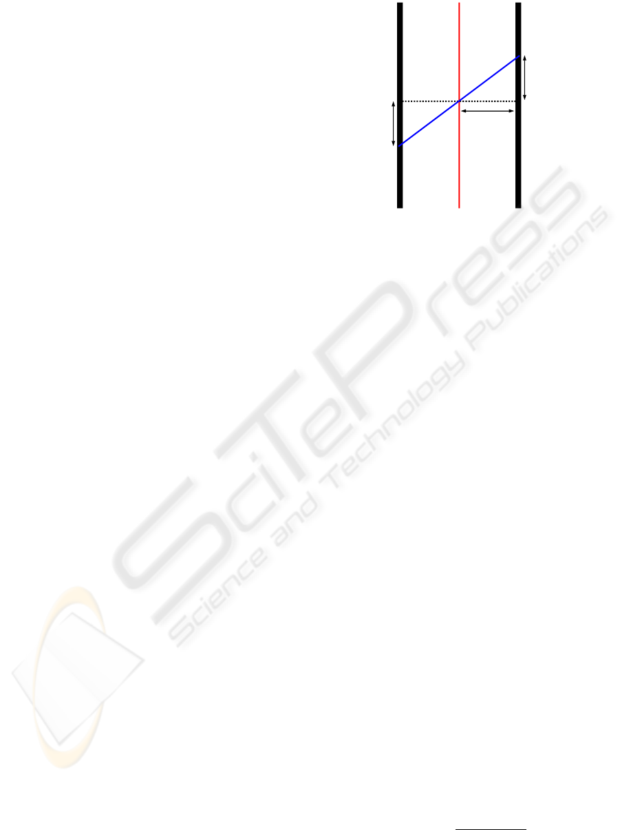
Figure 1: Illustration of slice registration setup and direction
of penalization vector field.
this by including a prior S in the cost function. That
is, a new approximation
˜
R is obtained by solving
min
˜
R
M [
˜
R,{S
k
}
k=1...K
] + βS
v
v
v
[
˜
R], (5)
where the coefficient β governs the effect of the prior.
In this work, we specifically consider a penalty
term that penalizes high image gradients in certain
directions. We write the prior as the inner product
between the gradient image and a vector field v
v
v, i.e.
S
v
v
v
[
˜
R] =
Z
Ω
h∇
˜
R(x
x
x),v
v
v(x
x
x)i
2
dx
x
x, (6)
That is, v
v
v determines the direction and magnitude of
the penalty – resulting in less regularization where the
two are approximately orthogonal and/or of low mag-
nitude. We call v
v
v the penalization vector field. The
following section presents a procedure for construct-
ing this vector field.
2.2 Constructing a Penalization Vector
Field
Inspired by (Penney et al., 2004; Frakes et al., 2008;
´
Olafsd
´
ottir et al., 2010) we obtain the penalization
vector field by non-rigid registration of neighboring
slices. We apply a symmetric registration between
slices, assuming that the point φ
φ
φ
1
(x
x
x) = x
x
x −u
u
u(x
x
x) in
slice S
1
corresponds to the point φ
φ
φ
2
(x
x
x) = x
x
x + u
u
u(x
x
x) in
slice S
2
. The concept is illustrated in Figure 1. The
penalization vector field is then composed by a half
slice thickness τ, the displacement u
u
u and a scale fac-
tor γ
v
v
v(x
x
x) = γ(x
x
x)
[τ, u
u
u(x
x
x)]
T
k[τ, u
u
u(x
x
x)]
T
k
. (7)
CAN ANISOTROPIC IMAGES BE UPSAMPLED?
77

The squared difference similarity measure drives
the registration as we assume that intensities in adja-
cent slices are directly comparable, and that the noise
is i.i.d., i.e.
D[S
1
,S
2
;u
u
u] =
Z
Ω
S
2
◦φ
φ
φ
2
(x
x
x) −S
1
◦φ
φ
φ
1
(x
x
x)
2
dx
x
x, (8)
with S
i
(φ
φ
φ
i
(x
x
x)) = S
i
◦φ
φ
φ
i
(x
x
x).
The free-form deformation model (Rueckert et al.,
1999) is used to model the deformation u
u
u in order to
reduce the dimensionality of the problem. Hence,
u
u
u(x
x
x; w
w
w) = hb
b
b(x
2
) ⊗b
b
b(x
1
),w
w
wi, (9)
where w
w
w are the deformation parameters, and b
b
b are
the B-splines.
To ensure a homeomorphic deformation we adapt
the Riemannian elasticity energy (Pennec et al., 2005)
in the registration process. The elasticity energy of a
deformation field φ
φ
φ is given by
S
rie
(φ
φ
φ) =
Z
Ω
µ tr(E
E
E
0
(x
x
x)
2
) +
λ
2
tr(E
E
E
0
(x
x
x))
2
dx
x
x (10)
where E
E
E
0
=
1
2
log((I
I
I + ∇φ
φ
φ)
T
(I
I
I + ∇φ
φ
φ)) is the Hencky
strain tensor.
Thus, correspondences between adjacent slices
are identified by solving
min
w
w
w
D[S
1
,S
2
;u
u
u] + α(S
rie
(φ
φ
φ
1
) + S
rie
(φ
φ
φ
2
)), (11)
where α determines the amount of regularization in-
troduced by the elasticity term.
Homogeneous areas in the image (e.g. back-
ground) contain no information to guide the registra-
tion. Therefore, one should be cautious when putting
great confidence in the local correspondences esti-
mated here. To address this issue we introduce an in-
formation score e for each registration point. This is
included by means of the scale factor γ of the penal-
ization vector field (7).
We base e on the edge information available in
the slice around each position, as edges within slices
are valuable in the registration. For a point x
x
x we fil-
ter around the position in the two neighboring image
slices φ
φ
φ
1
(x
x
x) and φ
φ
φ
2
(x
x
x) with the first order derivative
of a 1D Gaussian kernel (Canny, 1986)
G
0
σ
(x)
∂G
σ
(x)
∂x
=
−x
σ
1
σ
√
2π
exp−
x
2
2σ
2
. (12)
The kernel covers n pixels on each side of the pixel
and has a standard deviation of σ = n/3.
The score is then computed as the absolute value
of the sum of the two
e(x
x
x) =
G
0
σ
∗
S
1
◦φ
φ
φ
1
(x
x
x)
+ G
0
σ
∗
S
2
◦φ
φ
φ
2
(x
x
x)
. (13)
This means that both slices must contain edge infor-
mation around the matching point in order for the cor-
respondence to be regarded as strong.
The scale factor is then computed as the score di-
vided by a parameter ε plus the similarity measure of
(8)
γ(x
x
x) =
e(x
x
x)
ε + (S
2
◦φ
φ
φ
2
(x
x
x) −S
1
◦φ
φ
φ
1
(x
x
x))
2
. (14)
where the value of ε is related to the intensity level
of the image. As mentioned earlier, the penalization
vector field is then constructed by multiplying the cor-
respondence directions from the registration by these
scale factors.
3 EXPERIMENTS
In this section we present a study in 2D comparing our
proposed upsampling approach using the prior of the
penalization vector field (UPWP) against the standard
cubic interpolation (CI) (Keys, 1981) and the one-way
registration-based interpolation (RBI) (Penney et al.,
2004). For reference we also include a reconstruc-
tion performed using our method without the prior
(UPNP).
From a 250×250 isotropic-sampled Shepp-Logan
phantom (Shepp and Logan, 1974) we create a down-
sampled anisotropic image by averaging every five
columns together. Figures 2(a,b) show the isotropic
and anisotropic phantom. That is, the columns act as
the thick slices in the context described in the previous
section. Figure 2(c) displays the registration-based
line correspondences superimposed on the anisotropic
phantom. For the registration the knot spacing of
the B-splines was four pixels and the regularization
weight was 10
−2
. A penalization vector field was ex-
tracted from the registration. The columns were fil-
tered using the derivative of a 1D Gaussian kernel
with standard deviation
5
3
. The resulting field is dis-
played in Figure 2(d).
Four reconstructions were obtained from the
anisotropic-sampled phantom using CI, RBI and our
UPNP and UPWP without and with the penalization
vector field shown in Figure 2(d). Figure 3 contains
these reconstructions. For quantitative comparison
we computed the mean squared error (MSE) between
pixel values in the isotropic-generated phantom and
the reconstructions. Table 1 lists the results. From
Figure 3 and Table 1 we acknowledge that UPWP
VISAPP 2010 - International Conference on Computer Vision Theory and Applications
78
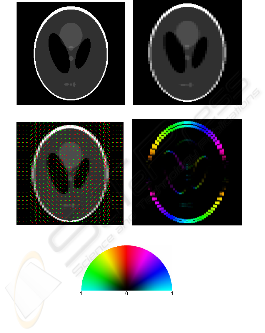
(a) Phantom. (b) Downsampled phantom.
(c) Downsampled phantom with correspondences
from the registration.
(d) Penalization vector field.
(e) Color-map for penalization vector field
field. The color shows the direction and the
brightness shows the magnitude.
Figure 2: Visualization of phantom data, symmetric registration and the penalization vector field.
provides the most visually pleasing result as well as
the lowest MSE. Finally, we see from Figure 3(b) that
the RBI approach provides visually nice interpolation
in areas with good registration, and unsatisfactory in-
terpolation in areas lacking correspondences – areas
where structures runs approximately parallel to the
slices. This problem and the method’s ability to re-
cover from partial volume effects of the upsampling
approach explain the lower MSE of our UPWP.
CAN ANISOTROPIC IMAGES BE UPSAMPLED?
79
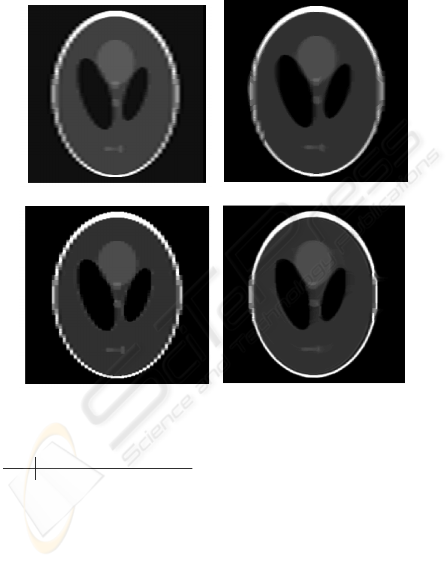
(a) Cubic interpolation. (b) One-way registration (Penney et al., 2004).
(c) Upsampling without prior. (d) Upsampling with prior.
Figure 3: Reconstructions.
Table 1: Mean squared error between reconstructions and
isotropic phantom for the four reconstruction methods.
CI RBI UPNP UPWP
MSE 0.0143 0.0073 0.0080 0.0045
4 CONCLUSIONS
This paper presented a novel approach for improv-
ing the resolution of anisotropic medical images. The
method relies on a prior constructed upon registra-
tions of neighboring slices. As such, the quality of the
prior is undoubtedly dependent on the quality of the
registrations. However, unlike the registration-based
interpolation method, it is possible to limit the effect
of mis-registrations by reducing the length of the pen-
alization vector field in areas with little information
or poor fit. The preliminary tests presented in the pa-
per showed promising results, motivating further in-
vestigation and validation.
REFERENCES
Canny, J. (1986). A computational approach to edge de-
tection. IEEE Transactions Pattern Analysis and Ma-
chine Intelligence, 8(6):679–698.
Frakes, D., Dasi, L., Pekkan, K., Kitajima, H., Sun-
dareswaran, K., Yoganathan, A., and Smith, M.
(2008). A New Method for Registration-based Medi-
cal Image Interpolation. IEEE Transactions on Medi-
cal Imaging, 27(3):370–377.
Gudbjartsson, H. and Patz, S. (1995). The rician distribution
VISAPP 2010 - International Conference on Computer Vision Theory and Applications
80

of noisy mri data. Magnetic Resonance in Medicine,
34(6):910–914.
Keys, R. G. (1981). Cubic Convolution Interpolation for
Digital Image Processing. IEEE Transactions on
Acoustics Speech and Signal Processing, 29(6):1153–
1160.
´
Olafsd
´
ottir, H., Pedersen, H., Hansen, M. S., Lyksborg, M.,
Darkner, S., and Larsen, R. (2010). Registration-based
Interpolation Applied to Cardiac MR. Proceedings of
SPIE Medical Imaging 2010: Image Processing.
Pennec, X., Stefanescu, R., Arsigny, V., Fillard, P., and Ay-
ache, N. (2005). Riemannian Elasticity: A Statis-
tical Regularization Framework for Non-linear Reg-
istration. Proceedings of the 8th International Con-
ference on Medical Image Computing and Computer-
Assisted Interventation (LNCS), 3750:943–950.
Penney, G., Schnabel, J., Rueckert, D., Viergever, M., and
Niessen, W. (2004). Registration-based Interpolation.
IEEE Transactions on Medical Imaging, 21(7):922–
926.
Rueckert, D., Sonoda, L. I., Hayes, C., Hill, D. L. G., Leach,
M. O., and Hawkes, D. J. (1999). Nonrigid Registra-
tion using Free-Form Deformations: Application to
Breast MR Images. IEEE Transactions on Medical
Imaging, 18(8):712–21.
Shepp, L. A. and Logan, B. F. (1974). The Fourier recon-
struction of a head section. IEEE Transactions on Nu-
clear Science, 21(3):21–43.
CAN ANISOTROPIC IMAGES BE UPSAMPLED?
81
