MARCHING CUBES IN AN UNSIGNED DISTANCE FIELD
FOR SURFACE RECONSTRUCTION FROM UNORGANIZED
POINT SETS
John Congote
1,2
, Aitor Moreno, I
˜
nigo Barandiaran, Javier Barandiaran, Jorge Posada
1
Vicomtech Research Center, Donostia - San Sebastian , Spain
Oscar Ruiz
2
CAD CAM CAE Laboratory, EAFIT University, Medellin, Colombia
Keywords:
Marching cubes, Surface reconstruction, Point set, Unsigned distance field.
Abstract:
Surface reconstruction from unorganized point set is a common problem in computer graphics. Generation
of the signed distance field from the point set is a common methodology for the surface reconstruction. The
reconstruction of implicit surfaces is made with the algorithm of marching cubes, but the distance field of a
point set can not be processed with marching cubes because the unsigned nature of the distance. We propose an
extension to the marching cubes algorithm allowing the reconstruction of 0-level iso-surfaces in an unsigned
distance field. We calculate more information inside each cell of the marching cubes lattice and then we
extract the intersection points of the surface within the cell then we identify the marching cubes case for the
triangulation. Our algorithm generates good surfaces but the presence of ambiguities in the case selection
generates some topological mistakes.
1 INTRODUCTION
Surface reconstruction from an unorganized point set
has been a widely studied problem in the computer
graphics field. The problem can be defined as given
a set of unorganized points which are near to a sur-
face. A new surface is reconstructed from that points.
Which is expected to be near to the original one.
Acquisition systems like laser scanners, depth es-
timation from images, range scan data, LIDAR and
other methodologies results in an unorganized point
set. Geometry analysis(Miao et al., 2005) and vi-
sualization process (Gross and Pfister, 2007) could
be done with this input, however the presence of
noise, out-layers or non scanned regions could gen-
erate problems in the reconstruction and analysis pro-
cess.
Reconstruction of the surface could be made in
several forms, like nurbs, polygonal meshes, implicit
or explicit functions. Triangular meshes are the most
common form of representation of surfaces. This rep-
resentation allows an easy extraction of the proper-
ties of the surface like curvatures, boundaries, and
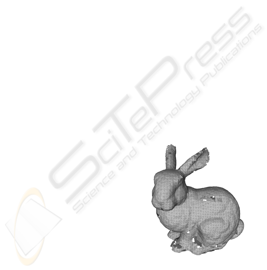
Figure 1: Reconstructed bunny model using marching
cubes in an unsigned distance field with a grid of 50
3
cells
with more than 140.000 points representing the surface.
other characteristics. Also the possibility of extension
from this output to visualization process are straight-
forward with the current graphic hardware.
143
Congote J., Moreno A., Barandiaran I., Barandiaran J., Posada J. and Ruiz O. (2010).
MARCHING CUBES IN AN UNSIGNED DISTANCE FIELD FOR SURFACE RECONSTRUCTION FROM UNORGANIZED POINT SETS.
In Proceedings of the International Conference on Computer Graphics Theory and Applications, pages 143-147
DOI: 10.5220/0002846901430147
Copyright
c
SciTePress
The contribution of this paper is the extension of
Marching Cubes algorithm by analyzing more infor-
mation inside each cell, for each edge inside the cell
the value of the middle point in the edge is calculated
as a other vertice. With the new information the in-
tersection points of the surface with the edges of the
cell are calculated, and the triangulation case for each
cell is selected generating the triangular surface of the
0-level iso-surface.
The remainder of the paper is structure as follows:
In section 2 we review previous work in surface re-
construction from point sets and their different ap-
proximations. In section 3 we present the methodol-
ogy of surface reconstruction of our algorithm. And
in section 4 we present the results of the algorithm
testing different quality measurements in the outputs
of the algorithm, conclusions and future work is pre-
sented in section 5.
2 RELATED WORK
Surface reconstruction from unorganized point set
has been solved with two different and predominant
methodologies. The first one is by Voronoi-Delone
and by implicit functions, the difference between the
methods are the base division of the process. Voronoi-
Delone the methods are point centric data calculation
process and the triangulation is created following the
point set. Implicit functions methodology divide the
space and the local characteristics of the surface in-
side are identifyied for further rendering with meth-
ods like Marching Cubes.
Reconstruction of surfaces with Voronoi-Delone
methodologies are explored in (Amenta et al., 1998)
where a 3D voronoi diagram is created of the point
set and a crust is generated. (Amenta et al., 2001) a
medial axis transform is calculated form the point set
and the surface is generated following the distance to
the medial axis.
Aproximation made by (Hoppe et al., 1992) which
for each point the normal direction is calculated using
the neighborhood of the point and then calculating the
tangent plane in that point with a least squares algo-
rithm. A consistent plane orientation for all the points
should be made assuring that all the point faces to the
same direction which is an NP problem. Finally a
signed distance function is generated and a triangular
mesh is generated with the marching cubes algorithm.
This methodology is improved in the work of (Kazh-
dan et al., 2006).
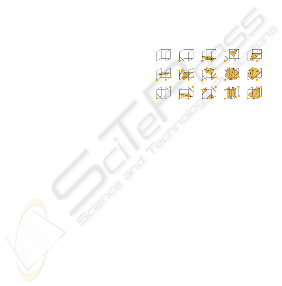
Marching cubes (Lorensen and Cline, 1987) is an
algorithm to generate triangular meshes from volu-
metric data. This algorithm defines a type of trian-
gulation for each cell in the volume or space given
the values of the vertices, given a desired iso-value
the vertices are compair against this value and then a
triangulation case is selected (Figure 2) and then a tri-
angulation is generated for each cell. The algorithm
has been widely studied (Newman and Yi, 2006)
and several extensions had been made to solve topo-
logical problems with techniques (Chernyaev, 1995),
(Lewiner et al., 2003) also methodologies to obtain
more accurate representations were studied (Congote
et al., 2009). One of the biggest advantages of the al-
gorithm is their complexity O(n) where n is the num-
ber of cells in the volume, so the time taken by the
algorithm to the process could be easily controlled in
real time process because it is constant and can be
modified changing the number of cells.
Figure 2: Marching Cubes cases.
The distance field generated from the set of points
represents a challenge for the marching cubes algo-
rithm because the distance is always a positive value,
and the surface which represents the points are de-
fined in the isovalue 0 which can not be represented
without the presence of negative values in the field.
To solve this problem a signed distance field must be
generated where, for each point in the set, the normal
of the surface is calculated, and must be congruent in
all the surface. This process is very complex and we
avoid this step in our work.
Previous approximations of modified marching
cubes algorithm from point sets has been made. (Fuji-
moto et al., 2008) which uses the vertices as the places
where the surface pass, to obtain better geometry ap-
proximation the vertices are translated to the nearest
point, and a new marching cubes cases are formulated
where the surface is in the vertices. (Hornung and
Kobbelt, 2006) creates an offset surface around the
points and then a cut between the offsets represent the
surface of the points.
3 METHODOLOGY
Our algorithm takes as input an unorganized point
set. A bounding box is created which contains the
set of points. A cubical grid is generated inside the
GRAPP 2010 - International Conference on Computer Graphics Theory and Applications
144

bounding box, where each vertex of the grid contains
the minimum distances from the vertex to the near-
est point of the point set. A parabolic interpolation
defines the points of intersection of the surface to the
grid. Then for each cell the marching cube case is
selected given the intersection points of the edges of
the cell. For each cell the triangles are generated with
following the marching cubes case obtaining the tri-
angular mesh which represent the surface of the point
set.
The problem as defined by (Hoppe et al., 1992)
takes as input an unorganized point set {x
1
, . . . , x
n
} ⊂
R
3
on or near an unknown manifold M, and recon-
struct a manifold M
0
which approximates M. No in-
formation about the manifold M as the presence of
boundaries or geometry of M are assumed to be knew
in advance.
Given a set of unorganized points P =
{p
1
, p
2
, . . . , p
n
} which are on or near to a mani-
fold δM, our goal is to construct a manifold δM
0
which are close to δM. Each point of P is represented
by a 3-tuple of real values. The manifold δM
0
is
represented as a set of planar triangles of R
3
The algorithm is subdivided in the following
steps:
1. Bounding box B calculation of P.
2. Generation of a cubical grid G inside B.
3. Calculate the minimum distance for each vertex
v
i, j,k
∈ G to P.
4. Calculate the intersection points I in the edges of
the cells of G.
5. Identify for each cell of G the marching cube case
which match the intersection points I.
6. Generate the simplexes of each cell of G given the
calculated case.
3.1 Bounding Box Calculation
The calculation of the bounding box B could be made
following the word axis identifying the minimum and
maximum values of (x, y, z) in P. There is no a exact
rule for the creation of the bounding box, which can
be parallel to the global axis, rotated or static. The
bounding box define the region in the space where the
triangular mesh is going to be generated.
3.2 Cubical Grid Generation
Inside the region defined by B a cubical grid G is de-
fined, the number of cells that are inside G define the
resolution of the surface, but a high number of cells
without a proper density of points defining the case
inside each cell could generate ambiguities in the re-
construction process. also the number of cells defines
the level of detail of the object. For each cell the ver-
tices of the grid are define as v, also a number of aux-
iliary vertices in the middle of each edge of the cell
must be created v
aux
.
Figure 3: Vertices v and auxiliary vertices v
aux
for each cell.
3.3 Distance Calculation for each Vertex
For all the vertices v and v
aux
defined in G the min-
imum distance from the vertex to the point cloud
should be calculated (Figure 3). Given the regular
form of the grid G for each point in P the nearest ver-
tex could be calculated in O(1) time, then the near
vertex is assigned with the value calculated, if various
points are near to the same vertex v then only then
minimum distance is stored.
3.4 Intersection Point Calculation
Edges of the cells C a possible intersection point is
calculated by Equation 1, where an intersection point
inside the edge is defined, this intersection point are
based with a tolerance value, which define if the point
is close enough to the edge to be defined as an inter-
section,
For each edge e of the cells C, we have 3 vertices,
v
1
, v
2
, v
3
where v
1
and v
3
are the vertices of the lat-
tices of the grid and v
2
is the middle auxiliary vertex
calculated v
aux
. Our methodology is to suppose that
vertices are aligned in the x axis in D plane with the
values of x
1
= 0, x
2
= 0.5 and x
3
= 1, and the values
of y
1
= v
1
, y
2
= v
2
, y
3
= v
3
which are a distance from
vertices to the surface point, are values in y axis of D
plane. Then we can assume that a normal signed sur-
face which cut the edge forms a line in the plane D,
as shown in Figure 4 but as the distance is a positive
value the intersection is presented as a line in the pos-
itive region of D. We approximate the intersection as-
MARCHING CUBES IN AN UNSIGNED DISTANCE FIELD FOR SURFACE RECONSTRUCTION FROM
UNORGANIZED POINT SETS
145
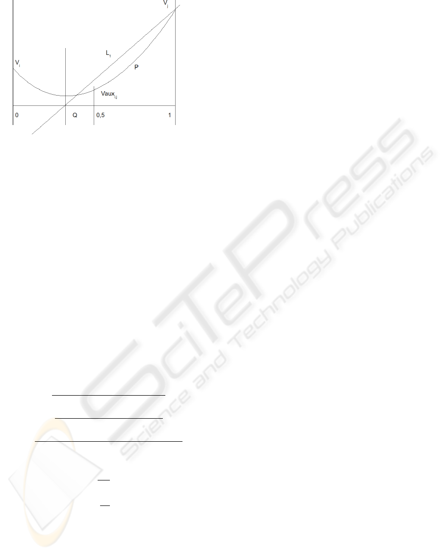
Figure 4: Parabola showing the intersetion point q for the
unsigned distance field as a comparison between the orig-
inal distance funcion L
1
and a parabola p which values v
i
,
v
j
, v
aux
represent the distance to the surface.
suming the as the intersection point can be expressed
as a parabola, which is aligned with the y axis in D.
Given the 3 points measured in the plane a parabola
p could be calculated solving the equations of 1 given
the parameters of p, a, b, c in Equation 2. v
x
, v
y
are the
coordinates of the vertice of the parabola p as defined
in Equation 3, the value v
x
gives the position in the
edge where the surface cuts the edge and v
y
could be
assigned as a tolerance value, which define how close
is the surface to the edge.
y
1
= ax
2
1
+ bx
1
+ c (1)
y
2
= ax
2
2
+ bx
2
+ c
y
3
= ax
2
3
+ bx
3
+ c
a = −
−x
2
y
1
+x
3
y
1
+x
1
y
2
−x
3
y
2
−x
1
y
3
+x
2
y
3
(x
2
−x
3
)(x
2
1
−x
2
x
1
−x
3
x
1
+x
2
x
3
)
(2)
b = −
y
2
x
2
1
−y
3
x
2
1
−x
2
2
y
1
+x
2
3
y
1
−x
2
3
y
2
+x
2
2
y
3
(x
1
−x
2
)(x
1
−x
3
)(x
3
−x2
)
c = −
x
3
y
2
x
2
1
−x
2
y
3
x
2
1
−x
2
3
y
2
x
1
+x
2
2
y
3
x
1
+x
2
x
2
3
y
1
−x
2
2
x
3
y
1
(x
2
−x
3
)(x
2
1
−x
2
x
1
−x
3
x
1
+x
2
x
3
)
v
x
=
−b
2a
(3)
v
y
= c −
b
2
4a
3.5 Cell Case Identification
Given the intersection points for each cell, the march-
ing cubes lookup table is used, to define which case of
marching cubes had the same edges intersected, if the
case is found then the cell is labeled with that case,
if there is not case which is defined by the marching
cubes look up table, then this cells had an ambigu-
ity case. These cases are produced because the points
around the cell had a lot of noise or there is no enough
density of points to identify the triangulation in that
region. At the time we don’t make any processing to
solve this ambiguity and that cells are simply are as-
signed as empty, but global process could be done to
eliminate this ambiguities.
3.6 Triangulation Generation
Each cell of the Grid G had been labeled with the
marching cubes case which represents. Then follow-
ing the rules of generation of triangles or simplexes of
marching cubes. The number of cases which march-
ing cubes gives is 14 in their original definition, be-
cause the number of possible combination of edges is
2
8
= 256 but eliminating redundant cases with rota-
tions or mirrors is only 14 cases. With out approach
the number of cases is equal to the number of possible
intersections of the edges 2
12
= 4096, where we map
to the 14 cases of marching cubes, as explained before
there is some configurations which gives ambiguity
forms this cases are not generated in our algorithm.
4 RESULTS
Our algorithm generates triangular mesh which is a
good representation of the surface defined by the set
of points. The mesh is not created to be correct
in a topological level because the original marching
cubes algorithm used to generate the triangulation
have topological errors, and the process of calcula-
tion is very sensitive to noise or poorly density re-
gions of points. The mesh is generated in a fast way.
Even though the results represent a qualitative good
representation of the surfaces. This algorithm focus
in the problem of generation of the surfaces without
the calculation of the normal direction of the surface
extending the uses of the Marching Cubes algorithm
for unsigned implicit functions in the representation
of the isolevel 0.
5 CONCLUSIONS AND FUTURE
WORK
We present an extension of the marching cubes al-
gorithm for the extraction of the 0-level iso-surface
in an unsigned distance field. The generated meshes
present a lot of topological mistakes because the al-
gorithm can not identify correctly the marching cubes
GRAPP 2010 - International Conference on Computer Graphics Theory and Applications
146
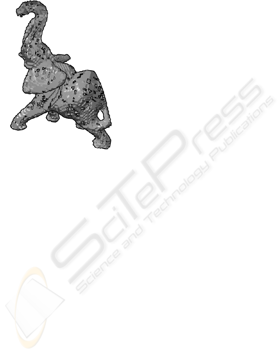
Figure 5: Reconstructed elephant model with a grid of 200
3
cells.
cases where the edges in the cell are intersected with a
different pattern as the marching cubes cases present.
New set of marching cubes cases have to be generated
to correct implement the triangulation step.
The algorithm could represent a big part of the
surface without calculating the normal, eliminating
an costly step commonly used in other algorithms
opening a new method for reconstruction for non-
orientable surfaces, and because the local nature of
the algorithm it can process without problems sur-
faces with holes or boundaries.
The quality of the meshes without considering the
errors produce by the ambiguieties are the same as
the marching cubes original algorithm. For futher
improvements in the quality of the meshes could be
applied using the different techniques developed for
marching cubes algorithm because the modification
of our extension to the original algorithm is minimal.
ACKNOWLEDGEMENTS
This work has been partially supported by the Spanish
Administration agency CDTI, under project CENIT-
VISION 2007-1007. CAD/CAM/CAE Laboratory -
EAFIT University and the Colombian Council for
Science and Technology – COLCIENCIAS –. The
data set of bunny is courtesy of the Stanford Com-
puter Graphics Laboratory.
REFERENCES
Amenta, N., Bern, M., and Kamvysselis, M. (1998). A new
voronoi-based surface reconstruction algorithm. In
SIGGRAPH ’98: Proceedings of the 25th annual con-
ference on Computer graphics and interactive tech-
niques, pages 415–421, New York, NY, USA. ACM.
Amenta, N., Choi, S., and Kolluri, R. K. (2001). The power
crust. In SMA ’01: Proceedings of the sixth ACM
symposium on Solid modeling and applications, pages
249–266, New York, NY, USA. ACM.
Chernyaev, E. V. (1995). Marching cubes 33: Construction
of topologically correct isosurfaces. Technical report,
CERN.
Congote, J. E., Moreno, A., Barandiaran, I., Barandiaran,
J., and Ruiz, O. (2009). Adaptative cubical grid for
isosurface extraction. In 4th International Confer-
ence on Computer Graphics Theory and Applications
GRAPP-2009, pages 21–26, Lisbon, Portugal.
Fujimoto, K., Moriya, T., and Nakayama, Y. (2008). Sur-
face reconstruction from high-density points using de-
formed grids. In WSCG’2008 Communication Papers
Proceedings, pages 117–120, Plzen - Bory, Czech Re-
public. University of West Bohemia.
Gross, M. and Pfister, H. (2007). POINT-BASED GRAPH-
ICS. Elsevier.
Hoppe, H., DeRose, T., Duchamp, T., McDonald, J., and
Stuetzle, W. (1992). Surface reconstruction from un-
organized points. In SIGGRAPH ’92: Proceedings
of the 19th annual conference on Computer graphics
and interactive techniques, pages 71–78, New York,
NY, USA. ACM.
Hornung, A. and Kobbelt, L. (2006). Robust reconstruction
of watertight 3d models from non-uniformly sampled
point clouds without normal information. In SGP ’06:
Proceedings of the fourth Eurographics symposium
on Geometry processing, pages 41–50, Aire-la-Ville,
Switzerland, Switzerland. Eurographics Association.
Kazhdan, M., Bolitho, M., and Hoppe, H. (2006). Pois-
son surface reconstruction. In SGP ’06: Proceedings
of the fourth Eurographics symposium on Geometry
processing, pages 61–70, Aire-la-Ville, Switzerland,
Switzerland. Eurographics Association.
Lewiner, T., Lopes, H., Vieira, A. W., and Tavares, G.
(2003). Efficient implementation of marching cubes’
cases with topological guarantees. journal of graph-
ics, gpu, and game tools, 8(2):1–15.
Lorensen, W. E. and Cline, H. E. (1987). Marching cubes:
A high resolution 3d surface construction algorithm.
SIGGRAPH Comput. Graph., 21(4):169–169.
Miao, Y., Feng, J., and Peng, Q. (2005). Curvature estima-
tion of point-sampled surfaces and its applications. In
Computational Science and Its Applications – ICCSA
2005, pages 1023–1032. Springer Berlin / Heidelberg.
Newman, T. S. and Yi, H. (2006). A survey of the marching
cubes algorithm. Computers & Graphics, 30(5):854–
879.
MARCHING CUBES IN AN UNSIGNED DISTANCE FIELD FOR SURFACE RECONSTRUCTION FROM
UNORGANIZED POINT SETS
147
