
4D MAP MRI IMAGE RECONSTRUCTION
Jacob Hinkle
1
, Ganesh Adluru
2
, Eugene Kholmovski
2
, Edward DiBella
2
and Sarang Joshi
1
1
Scientific Computing and Imaging Institute, University of Utah, Salt Lake City, Utah, U.S.A.
2
Utah Center for Advanced Imaging Research, University of Utah, Salt Lake City, Utah, U.S.A.
Keywords:
MRI, Reconstruction, Motion, Diffeomorphic.
Abstract:
Conventional MRI reconstruction techniques are susceptible to artifacts when imaging moving organs. In
this paper, a reconstruction algorithm is developed that accommodates respiratory motion instead of using
only navigator-gated data. The maximum a posteriori (MAP) algorithm uses the raw k-space time-stamped
data and the 1D diaphragm navigator signal to reconstruct the images and estimate deformations in anatomy
simultaneously. The algorithm eliminates blurring due to binning the data and increases signal-to-noise ratio
(SNR) by using all of the collected data. The algorithm is tested in a simulated torso phantom and is shown to
increase image quality by dramatically reducing motion artifacts.
1 INTRODUCTION
Conventional MRI reconstruction techniques are sus-
ceptible to artifacts when imaging moving organs.
Navigators are often used in MRI to handle respira-
tory motion. The navigator rapidly images a 1D “pen-
cil” perpendicular to the diaphragm. This gives a 1D
signal in which the position of the diaphragm in the
superior-inferior direction can be found in nearly real-
time. In the heart, part of the k-space of the image is
acquired following each navigator for a brief period
corresponding to cardiac diastole. Diastole is defined
by the electrocardiogram (ECG) signal from the sub-
ject. This k-space data is marked to be used if the po-
sition of the diaphragm is within an acceptance win-
dow set by the user. Otherwise, that portion of k-space
is re-acquired during the next heartbeat. The naviga-
tor is repeated each heartbeat, as is the collection of
part of the image k-space, until all of k-space is ac-
quired and marked usable. This respiratory gating al-
gorithm can prolong the acquisition significantly. In-
creasing the acceptance window shortens acquisition
time but leads to image blurring.
In this paper, we take an alternate approach by
developing a reconstruction algorithm that accommo-
dates motion instead of discarding k-space data ac-
quired when the diaphragm position is outside the ac-
ceptance window. The maximum a posteriori (MAP)
algorithm uses raw time-stamped data to reconstruct
the images and estimate deformations in anatomy
simultaneously. The algorithm eliminates artifacts
by avoiding gating processes and increases signal-to-
noise ratio (SNR) by using all of the collected data.
This framework also facilitates the incorporation of
fundamental physical properties such as the conser-
vation of local tissue volume during the estimation of
the organ motion.
Previous attempts at reducing motion artifacts do
not offer all the advantages of our proposed method,
which incorporates a fully diffeomorphic motion
model into the reconstruction process. As early as
1991, Song and Leahy (Song and Leahy, 1991) used
an incompressible optical flow method for image reg-
istration. Rohlfing et al. (Rohlfing et al., 2003) use a
spline-based model which penalizes tissue compres-
sion to perform incompressible image registration.
Saddi et al. (Saddi et al., 2007) study incompressible
fluid-based registration. Their approach requires so-
lution of Poisson’s equation via a multigrid method
at each iteration. Despite these efforts in image reg-
istration, the incompressible nature of internal organs
has not previously been incorporated into the image
reconstruction process.
Here we test the feasibility of the new framework
on a phantom generated from 3D late gadolinium en-
hancement imaging of the left atrium (McGann et al.,
2008).
251
Hinkle J., Adluru G., Kholmovski E., DiBella E. and Joshi S. (2010).
4D MAP MRI IMAGE RECONSTRUCTION.
In Proceedings of the International Conference on Computer Vision Theory and Applications, pages 251-257
DOI: 10.5220/0002847102510257
Copyright
c
SciTePress

2 4D MAP IMAGE
RECONSTRUCTION
In conventional magnetic resonance imaging a pulse
sequence is designed in order to sample the Fourier
transform (k-space) of a 3D image. After acquiring
enough data to fill a Cartesian grid, an image I(x) is
reconstructed by performing an inverse Fourier trans-
form on the data. Such a method is justified when
imaging a static subject. However, severe artifacts are
introduced when the patient’s anatomy undergoes de-
formation during the scan.
Instead of avoiding motion artifacts in order to im-
prove image quality, we seek to understand motion
by modeling and estimating a four-dimensional image
I(t,x). Our method extends that of Hinkle et al. (Hin-
kle et al., 2009) thatp operates on real tomographic
projection data to complex-valued MRI data. The al-
gorithm is described in detail in the following sec-
tions.
2.1 MRI Data Acquisition Model
In MRI data acquisiton, values of the Fourier trans-
form of I(t,x) are sampled directly:
F {I}(ω) =
1
(2π)
3/2
Z
Ω
I(x)e
−iω·x
dx,
where Ω ⊂ R
3
is the image domain. Note that both
I(x) and F {I}(ω) are complex numbers. We model
our collected data as a collection of sets of measure-
ments of F {I}(ω) for different values of ω. These
sets consist of samples which were acquired within
a very short time of one another so that the anatomy
is in the same configuration for all samples from the
same set. For example, for a Cartesian sampling
scheme in which a single line of k-space is obtained
at each echo, a set of data consists of all the sam-
pled k-space values along that line. In general, the set
of sampled points may lie along a single line, mul-
tiple lines, or on some other curve for more exotic
sampling schemes. We will denote the sampled sets
of k-space locations as Ω
i
and their measured values
d
i
(ω),ω ∈ Ω
i
.
Since actual data is contaminated by noise, we
model each data point d
i
(ω) as a sample of a nor-
mal distribution with mean F {I(t
i
,x)}(ω) and some
variance σ
2
. If I(t, x) is the true 4D image, the log-
likelihood of observing the data is
L({d
i
}|I) =
−
1
2σ
2
N
∑
i=1
Z
Ω
i
kF {I(t
i
,x)}(ω) − d
i
(ω)k
2
C
dω.
(1)
2.2 Motion Model
Having modeled the data acquisition and noise, we
could attempt to estimate a 4D image I(t, x) which
maximizes the data log-likelihood. Indeed this is the
basis of many static reconstruction algorithms which
estimate I(x) in order to best fit the data. However,
in our case the additional temporal dimension of our
image domain forces us either to collect much more
data or to make use of some other information.
We model the 4D image as a single 3D image
I
0
∈ L
2
(Ω) undergoing a time-indexed deformation
h : [0, T ] × Ω → Ω. In this formulation I(t, x) is writ-
ten as I
0
◦ h(t,x). The problem at hand is then to es-
timate both the base image and motion which best fit
the data.
The estimated time-indexed deformation is meant
to model the motion of real tissue. It is useful to intro-
duce a prior on the motion estimates in order to esti-
mate deformations that are consistent with real tissue
and organ properties. One possibility is to model the
time-indexed deformation as a fluid flow. The defor-
mation is then fully determined by a set of velocity
fields v(t, x), which are defined as
v(t, x) =
d
dt
h(t, x).
Note that given this set of velocity fields the deforma-
tion can be recovered by integration:
h(t, x) = x +
Z
t
0
v(τ,h(τ,x))dτ
If the velocity fields are all smooth spatially then
the resulting integral field is guaranteed to be a diffeo-
morphism. As organs are not expected to tear apart
or drastically change geometry during physiological
motion, this is a reasonable requirement for many 4D
imaging applications. In order to enforce this prop-
erty, a formal prior is placed on the velocity fields in
the form of an inner product norm,
kvk
2
V
= hv,vi
V
=
Z
T
0
Z
Ω
kLv(t, x)k
2
R
3
dxdt,
where L is a differential operator chosen to reflect
physical tissue properties. In our implementation, L is
defined by Lv = −α∇
2
v − β∇∇ · v + γv for scalar pa-
rameters α,β, and γ. Although in this work we have
used a homogeneous operator, L could be spatially-
varying reflecting the different material properties of
the underlying anatomy.
As discussed, the problem is ill-posed if we do
not have an abundance of data. In such a case we
need to make further assumptions. Many 4D scan-
ning protocols make use of a navigator echo as a
signal indicating respiratory motion. If the signal is
VISAPP 2010 - International Conference on Computer Vision Theory and Applications
252

well-correlated with the internal anatomical configu-
ration, it may be used to reduce the data requirements
for the 4D reconstruction problem. If a signal, a(t),
is a faithful surrogate of the internal anatomy, then
a(t
1
) = a(t
2
) implies that I(t
1
,x) = I(t
2
,x). This is
satisfied if h(t
1
,x) = h(t
2
,x) for all x. This will be
true for all times with matching surrogate signal am-
plitudes, so it is convenient to index the deformations
by amplitude instead of time. Formally, we will write
h(t, x) = h(a(t),x).
Returning to the definition of v(t,x) the change of
variables looks like
v(t, x) =
d
dt
h(a(t), x) = v(a(t),h(a(t), x))
da
dt
,
where v(a,x) is a velocity field with respect to
changes in surrogate signal instead of time. The de-
formation to any amplitude is then obtained by the
integration of Eq. 2.2,
h(a,x) = x +
Z
a
0
v(a
0
,h(a
0
,x))da
0
.
The motion prior is modified accordingly by replac-
ing the time-indexed velocities with these amplitude-
dependent ones:
kvk
2
V
= hv,vi
V
=
Z
1
0
Z
Ω
kLv(a,x)k
2
R
3
dxda.
When modeling organs such as liver which are es-
sentially incompressible during normal activity, unre-
alistic deformations may be easily recognized if they
represent local compression or expansion. Estima-
tion of these types of unrealistic deformations may
be avoided by constraining the deformations to be in-
compressible. Deformations defined as a flow along
smoothly-varying vector fields as described in Eq. 2.2
have been well studied (Arnold, 1997). In particular,
if the divergence of the velocity field is zero the re-
sulting deformation is guaranteed to preserve volume
locally and have unit Jacobian determinant. It will be
useful to enforce this constraint in our algorithm when
modelling incompressible tissue.
2.3 Posterior Likelihood and
Optimization
The data log-likelihood and motion prior are com-
bined to give the posterior log-likelihood,
L(I
0
,v|d
i
) = − kvk
2
V
−
1
2σ
2
N
∑
i=1
Z
Ω
i
kF {I
0
◦ h(a
i
,·)}(ω) − d
i
(ω)k
2
C
dω.
(2)
The 4D image reconstruction problem is to es-
timate the image and velocity fields that maximize
Eq. 2,
(
ˆ
I
0
, ˆv) = argmax
I
0
,v
L(I
0
,v|d
i
) subject to divv = 0.
A MAP estimate (one that maximizes Eq. 2) is ob-
tained via an alternating iterative algorithm which at
each iteration updates the estimate of the deformation
in a gradient ascent step then updates the image.
The continuous amplitude-indexed velocity field
is discretized by a set of equally-spaced amplitudes
a
k
with the associated velocities v
k
, with spacing ∆a.
Note that this amplitude discretization is independent
of the amplitudes at which data is acquired. The de-
formation from amplitude a
k
to a
k+1
is approximated
by the Euler integration of Eq. 2.2,
h(a
k+1
,x) = h(a
k
,x) + v
k
(h(a
k
,x))
and the deformation for an amplitude a
i
between a
k
and a
k+1
is linearly interpolated as
h(a
i
,x) = h(a
k
,x) +
a
i
− a
k
∆a
v
k
(h(a
k
,x)).
Note that higher order integration schemes such as
Runge-Kutta may also be used in place of the simpler
Euler method.
The first variation of Eq. 2 with respect to v
k
under
the inner product in Eq. 2.2 is given by
δ
v
k
L(I
0
,v
k
,x|d
i
) = −2v
k
(x)
−
1
σ
2
(L
†
L)
−1
N
∑
i=1
Re[g
i
(x)b
i
(k, x)
∗
],
(3)
where g
i
(x) = F
−1
(F {I
0
◦ h(a
i
,·)} − d
i
)(x) and b
i
is
the contribution to the variation due to data set i, de-
fined as follows.
Let I
k
(x) = I
0
◦ h(a
k
,x) be the 3D reference image
pushed forward to amplitude a
k
. Then the factors b
i
are given by
b
i
(k, x) =
0 a
i
≤ a
k
a
i
−a
k
∆a
∇I
k
(x +
a
i
−a
k
∆a
v
k
(x)) a
k
< a
i
≤ a
k+1
J
i,k+1
∇I
k
(x + v
k
(x)) a
i
> a
k+1
,
where J
i,k+1
is the Jacobian determinant of
the transformation from amplitude a
i
to a
k+1
,
D(h
a
k+1
◦ h
−1
a
i
)(x)
. If the deformations are con-
strained to be incompressible, implying that the
Jacobian determinant is unity, this simplifies to
b
i
(k, x) =
0 a
i
≤ a
k
a
i
−a
k
∆a
∇I
k
(x +
a
i
−a
k
∆a
v
k
(x)) a
k
< a
i
≤ a
k+1
∇I
k
(x + v
k
(x)) a
i
> a
k+1
.
4D MAP MRI IMAGE RECONSTRUCTION
253
0 10 20 30 40 50
−50
−45
−40
−35
−30
Heart Beat
0 10 20 30 40 50
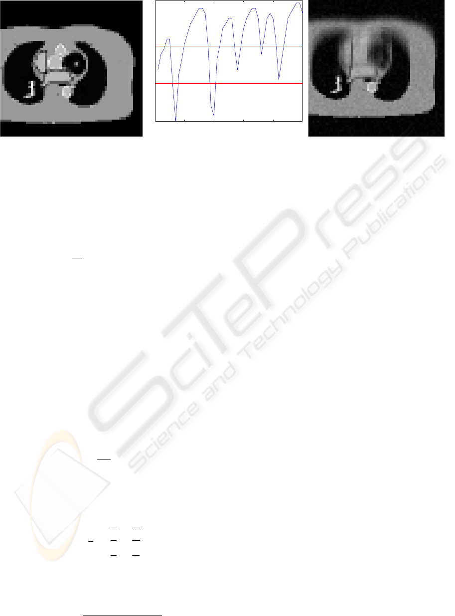
Figure 1: Static phantom (left), breathing signal from real patient navigator echo used in simulation with red lines indicating
boundary between bins used in binning method (center), and static 3D reconstruction of data from moving phantom (right).
Following the approach of Beg et al. (Beg et al.,
2005), efficient computation of (L
†
L)
−1
is imple-
mented in the Fourier domain, requiring only a matrix
multiplication and Fourier transforms of v
k
at each it-
eration of the algorithm.
The first variation of Eq. 2 with respect to I
0
is
δ
I
0
L(I
0
,v,x|d
i
) =
1
σ
2
∑
i
|Dh
−1
(a
i
,x)|g
i
(x) ◦ h
−1
(a
i
,x).
(4)
With these variations a gradient descent algorithm
can be implemented. However, as discussed previ-
ously, it is sometimes useful to enforce further tissue
constraints. The Helmholtz-Hodge decomposition al-
lows us to implement the incompressibility constraint
by simply projecting the unconstrained velocity fields
onto the space of divergence-free vector fields at each
iteration of the algorithm (Cantarella et al., 2002). In
order to efficiently implement the Helmholtz-Hodge
decomposition of a time-varying velocity field, we
use the discrete divergence operator as it operates
in Fourier domain. We write the discrete Fourier
transform of a central difference approximation to the
derivative of a function f as
DFT
{
∆
x
f
}
(ω) =
i
2k
x
sinωDFT
{
f
}
(ω).
In the Fourier domain the divergence of a vector field
takes the following form:
DFT
{
divv
}
(ω) = W (ω) · DFT
{
v
}
(ω),
where
W (ω) =
i
2
1
k
x
sin
ω
x
N
x
1
k
y
sin
ω
y
N
y
1
k
z
sin
ω
z
N
z
.
This allows us to remove the divergent component
easily in Fourier space via the projection
DFT
{
v
}
(ω) 7→ DFT
{
v
}
(ω)
−
W (ω) · DFT
{
v
}
(ω)
kW (ω)k
2
C
3
W (ω).
(5)
I
0
← 0
for each k do
v
k
← 0
end for
repeat
I
0
← I
0
+ εδ
I
0
L(I
0
,v)
for each k do
v
k
← v
k
+ εδ
v
k
L(I
0
,v
k
)
v
k
← Perform divergence-free projection on v
k
(optional)
end for
until algorithm converges or maximum number it-
erations reached
Figure 2: Pseudocode for 4D reconstruction.
Since the operator (L
†
L)
−1
is implemented in the
Fourier domain there is little computational overhead
in performing this projection at each iteration of the
algorithm.
Note that as soon as the velocity field is updated,
the image estimate must also be updated. The change
of image estimate in turn alters the velocity gradients
leading to a joint estimation algorithm in which, at
each iteration, the velocity fields are updated and then
the image recalculated.
Figure 2 summarizes the 4D reconstruction proce-
dure. The velocity fields are initialized to zero, so that
the initial estimate of the base image is simply the re-
sult of averaging all of the data. This yields a quite
blurry image that sharpens upon further iterations as
the motion estimate improves.
3 RESULTS
A realistic 3D phantom was created from a late
gadolinium enhancement (LGE) acquisition of a post-
ablation patient (Peters et al., 2007; McGann et al.,
2008) acquired on a Siemens Verio 3T scanner. Reso-
VISAPP 2010 - International Conference on Computer Vision Theory and Applications
254
lution was 1.25x1.25x2.5mm and 40 slices were ac-
quired. 19 different structures were manually seg-
mented and assigned different T1 values. The inver-
sion time was chosen to null myocardial signal. A
single slice was extracted to test the MAP image re-
construction method. This slice was downsampled to
60x60 pixels and k-space measurements of the slice
were simulated as 30 phase encodes per heartbeat.
Each set of 30 phase encodes was subjected to a de-
formation. The deformation was designed to simulate
the motion of the torso during breathing. The spine
and back stayed stationary while the chest wall and
anterior portion of the torso moved in the anterior di-
rection. The motion was designed to be proportional
to a breathing signal a(t) which was extracted from a
navigator echo of the patient. Both the 2D phantom
and the respiratory signal used to generate the defor-
mations are shown in Fig. 1.
A static reconstruction of the simulated data was
performed by averaging the recorded values at each
point in k-space then performing an inverse discrete
Fourier transform on the resulting 2D grid. Figure 1
shows the resulting image. Notice the extreme blur-
ring artifacts caused by averaging all of the collected
data while ignoring motion.
The breathing signal was then used to bin the sim-
ulated k-space data into three bins. The boundaries
between bins are displayed as red lines in Fig. 1. Note
that the bottom bin has very few data points. The re-
sult is that this bin cannot be reliably reconstructed.
This illustrates a major difficulty associated with bin-
ning or gating. The comparisons that follow will deal
only with the top two bins, in which there is enough
data that the binning method might have a realistic
chance of producing an image.
A 4D MAP reconstruction was also performed on
the same data. The static phantom, static reconstruc-
tion of moving phantom, and 4D MAP reconstruction
of moving phantom are shown in Fig. 4. Notice the
improvement in image quality. In particular, the 4D
MAP reconstruction avoids the blurring of edges seen
in the static reconstruction. Also note the decreased
noise in the 4D MAP reconstructed images as com-
pared to the binned images. This illustrates the ad-
vantages of techniques which use all of the data, such
as 4D MAP reconstruction, as opposed to gating or
binning. For comparison purposes, only two images
are shown of the 4D MAP reconstruction. However,
images can easily be generated corresponding to any
breathing amplitude. This contrasts gating and bin-
ning procedures, in which more data needs to be ac-
quired in order to generate more images.
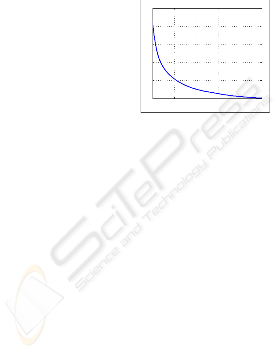
Figure 3 shows a plot of the objective function,
Eq. 2, as the algorithm ran. Note that the shape of
0 2000 4000 6000 8000 10000
2
3
4
5
6
7
x 10
4
Iteration
Energy
Figure 3: Convergence plot showing that the posterior like-
lihood has been minimized.
the plot indicates that the algorithm has converged.
This algorithm employs a gradient descent method,
as discussed previously. However, many optimization
schemes exist which could replace this simple method
and possibly offer faster convergence.
In addition to improving the image estimates, a
valuable motion estimate is also obtained during 4D
reconstruction. Figure 5 shows a comparison of the
true deformation applied to the phantom in order to
generate the data and that obtained by the 4D MAP
reconstruction algorithm. Note that the fully high-
dimensional deformation has been estimated quite ac-
curately. The algorithm is of course not able to reli-
ably estimate motion in areas where the image is ho-
mogeneous, as indicated by the slight deviations near
the right and left edges of the image.
4 CONCLUSIONS
A 4D reconstruction method was shown to reduce
motion artifacts in simulation. Instead of avoiding
motion effects by discarding data acquired when the
diaphragm was not within an acceptance window, the
method estimates the motion directly from all of the
raw data. The method was shown to reduce blurring
artifacts in a two-dimensional phantom. In addition,
SNR was improved. These are critically important
considerations for many respiratory-gated MRI stud-
ies. Not only were the images improved but a valu-
able motion estimate was obtained. This motion esti-
mate was shown to be accurate in regions where the
anatomy has sufficient contrast to enable tracking of
tissue.
The results in this paper were implemented in
4D MAP MRI IMAGE RECONSTRUCTION
255
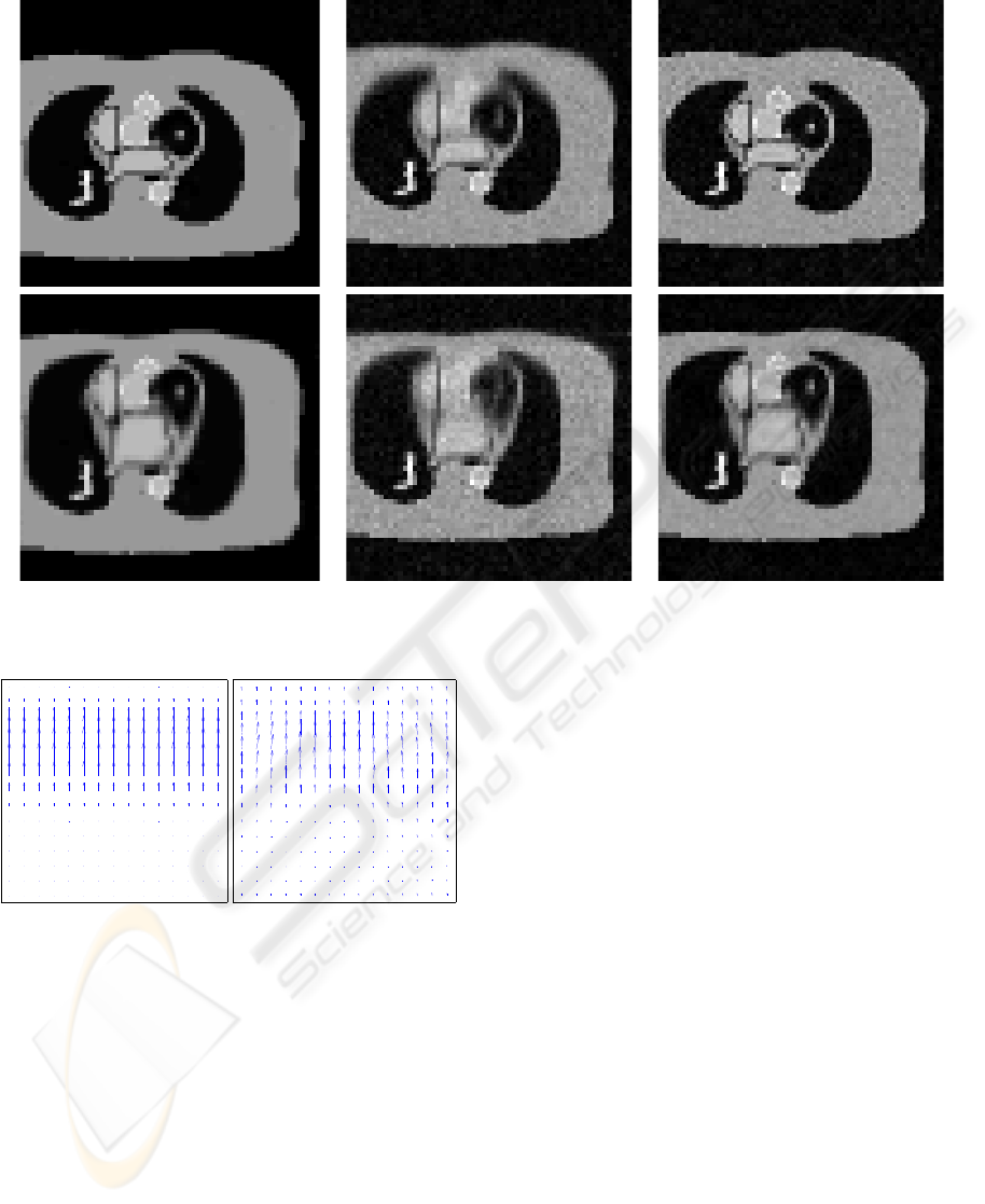
True Binning 4D MAP
Figure 4: True phantom along with binned and 4D MAP reconstructed images. The top row shows reconstructions at
amplitude a = 1, while the bottom row shows reconstructions at amplitude a = 0.5.
Figure 5: The true velocity field used to generate simulated
data (left) and the motion estimate resulting from 4D MAP
reconstruction (right).
MATLAB using a 2D version of the algorithm. The
method will be extended to real 4D data from MRI of
patients being treated for atrial fibrillation. Current
efficiencies of the respiratory navigator scan range
from 20% to 60%, implying the methods here could
substantially improve the image quality and/or allow
for a more rapid scan by using a larger acceptance
window.
The move to true 4D reconstruction is conceptu-
ally trivial, but will introduce added computation, as
the amount of lines will increase as well as the size
of the estimated images and velocity fields. However,
the algorithm lends itself particularly well to parallel
computation which should allow even the full 3D im-
plementation to run in a reasonable amount of time.
The intent of this work is to introduce a framework
by which 4D data was reconstructed using a motion
surrogate signal. The framework is flexible and could
be extended for other applications. The motion signal
was extracted from a navigator echo sequence, giving
a direct measure of internal anatomy. However, if a
navigator echo is unsuitable for a particular scan, an-
other respiratory signal could be used, such as a chest
marker or spirometer. Also, if enough data is avail-
able the motion surrogate could be ignored and time-
indexed deformations estimated.
There are other possible extensions to the algo-
rithm presented in this paper. For instance, if an
artifact-free base image is available, this can be di-
rectly used to obtain a best fit deformation estimate.
The reconstruction algorithm also does not dictate
what k-space trajectory to use. A Cartesian sampling
scheme was simulated in this work but other trajec-
tories such as spiral and polar acquisitions could be
used with very little modification to the algorithm.
VISAPP 2010 - International Conference on Computer Vision Theory and Applications
256

REFERENCES
Arnold, V. I. (1997). Mathematical Methods of Classical
Mechanics. Springer, 2nd edition.
Beg, M. F., Miller, M. I., Trouv
´
e, A., and Younes, L.
(2005). Computing large deformation metric map-
pings via geodesic flows of diffeomorphisms. Int. J.
Comp. Vis., 61(2):139–157.
Cantarella, J., DeTurck, D., and Gluck, H. (2002). Vec-
tor calculus and the topology of domains in 3-space.
Amer. Math. Monthly, 109(5):409–442.
Hinkle, J., Fletcher, P. T., Wang, B., Salter, B., and Joshi, S.
(2009). 4D MAP image reconstruction incorporating
organ motion. In IPMI 2009: Proceedings of Informa-
tion Processing in Medical Imaging, pages 676–687.
McGann, C. J., Kholmovski, E. G., Oakes, R. S., Blauer,
J. J., Daccarett, M., Segerson, N., Airey, K. J., Akoum,
N., Fish, E., Badger, T. J., DiBella, E. V., Parker, D.,
MacLeod, R. S., and Marrouche, N. F. (2008). New
magnetic resonance imaging-based method for defin-
ing the extent of left atrial wall injury after the abla-
tion of atrial fibrillation. J Am Coll Cardiol, 52:1263–
1271.
Peters, D. C., Wylie, J. V., Hauser, T. H., Kissinger, K. V.,
Botnar, R. M., Essebag, V., Josephson, M. E., and
Manning, W. J. (2007). Detection of pulmonary
vein and left atrial scar after catheter ablation with
three-dimensional navigator-gated delayed enhance-
ment MR imaging: Initial experience. Radiology,
243:690–695.
Rohlfing, T., Calvin R. Maurer, J., Bluemke, D. A., and
Jacobs, M. A. (2003). Volume-preserving nonrigid
registration of MR breast images using free-form de-
formation with an incompressibility constraint. IEEE
Trans. Med. Imag., 22(6):730–741.
Saddi, K. A., Chefd’hotel, C., and Cheriet, F. (2007). Large
deformation registration of contrast-enhanced images
with volume-preserving constraint. In Proceedings of
International Society for Optical Engineering (SPIE)
Conference on Medical Imaging 2007, volume 6512.
Song, S. M. and Leahy, R. M. (1991). Computation of 3-D
velocity fields from 3-D cine CT images of a human
heart. IEEE Trans. Med. Imag., 10(3):295–306.
4D MAP MRI IMAGE RECONSTRUCTION
257
