TEMPORAL PHOTON DIFFERENTIALS

L. Schjøth

, J. R. Frisvad

, K. Erleben

and J. Sporring

eScience Center, Department of Computer Science, University of Copenhagen, Denmark

Department of Informatics and Mathematical Modelling,Technical University of Denmark, Denmark

Keywords:

Photon mapping, Ray differentials, First order structure.

Abstract:

The ﬁnite frame rate also used in computer animated ﬁlms is cause of adverse temporal aliasing effects. Most

noticeable of these is a stroboscopic effect that is seen as intermittent movement of fast moving illumination.

This effect can be mitigated using non-zero shutter times, effectively, constituting a temporal smoothing of

rapidly changing illumination. In global illumination temporal smoothing can be achieved with distribution ray

tracing (Cook et al., 1984). Unfortunately, this, and resembling methods, requires a high temporal resolution

as samples has to be drawn from in-between frames. We present a novel method which is able to produce high

quality temporal smoothing for indirect illumination without using in-between frames. Our method is based

on ray differentials (Igehy, 1999) as it has been extended in (Sporring et al., 2009). Light rays are traced as

bundles creating footprints, which are used to reconstruct indirect illumination. These footprints expand into

the temporal domain such that light rays interacting with non-static scene elements draw a path reacting to the

elements movement.

1 INTRODUCTION

Rendering animated scenes with global illumina-

tion methods produces some interesting problems,

where the perhaps most prominent problem is alias-

ing caused by the fact that the temporal domain is

discretized at a often very low resolution.

Feature ﬁlms usually shot a frame rate around 25

frames per second (fps). Despite the fact that the hu-

man eye is much more perceptible than 25 fps, this

frame rate still gives a seemingly ﬂuid motion when

a ﬁlm is produced with a traditional movie camera.

However, were we to produce a feature ﬁlm of an an-

imated virtual scene using an unmodiﬁed global illu-

mination method at a frame rate of 25 fps, ﬂuid mo-

tion is not guaranteed. A typical unmodiﬁed global

illumination method produces images at instant time

in the temporal domain. This procedure can induce

temporal aliasing, which is seen as an adverse strobo-

scopic effect, where the illumination changes rapidly

over time. A traditional-camera produced feature

ﬁlm will avoid this problem because the camera has

non-zero exposure time. This means that camera-

perceived illumination is averaged over the exposure

time. In effect, high frequency motion is blurred and

therefore seems ﬂuid. This effect is often called mo-

tion blur. A temporal aliasing defect not solved by

this blurring is the wagon-wheel effect, which is seen

as a backwards turning of the spokes of a wheel due

to temporal under sampling. However, as our method

does not address this particular problem, it will not be

discussed further here. A survey paper for global illu-

mination and rendering solutions exploiting temporal

coherence is given in (Tawara et al., 2004).

Brute force methods, such as the accumulation

buffer (Haeberli and Akeley, 1990), average together

in-between frames in order to achieve motion blur.

These methods can achieve arbitrary high accuracy

but are often prohibitively expensive as full render-

ings typically have to be made of a large number of

in-between frames.

Different global illumination methods also ad-

dress temporal aliasing by simulating motion blur.

Distribution ray tracing (Cook et al., 1984) achieves

motion blur by stochastically sampling the temporal

domain as well as the spatial. In (Myszkowski et al.,

2001) the authors adaptively controlled the tempo-

ral and spatial sampling resolution by examining lo-

cal variations of indirect illumination over time and

space in a pilot estimate. In (Egan et al., 2009) motion

blur is modeled as a wedge in the frequency domain.

Ray tracing methods using ray differentials have been

studied in (Igehy, 1999; Christensen et al., 2003; Du-

rand et al., 2005; Gjøl et al., 2008).

Schjøth L., R. Frisvad J., Erleben K. and Sporring J. (2010).

TEMPORAL PHOTON DIFFERENTIALS.

In Proceedings of the International Conference on Computer Graphics Theory and Applications, pages 54-61

DOI: 10.5220/0002847800540061

 SciTePress

With time dependent photon mapping (Cam-

marano and Jensen, 2002), photon mapping was ex-

tended such that indirect illumination was estimated

using a four dimensional photon map that expanded

into the temporal domain. In this manner photons

were ﬁltered not only based on their spatial position

but also their temporal.

A problem common to the discussed methods is

that they all rely on information from in-between

frames in order to achieve motion blur. Having this

information available places certain restrictions on the

animated scene; because a scene description is needed

at arbitrary time steps, movement of scene elements

either needs to be described as a an analytic function,

or movement has to be interpolated between frames.

The analytical approach is by far the best but demands

a certain complexity of the animation application, as

well as a tight link to the rendering software. The

interpolative approach is error prone, since the ani-

mation curve might not be linear. Furthermore, some

accelerator for ray-object intersection (such as a bsp-

tree) typically needs to be either rebuild, or at least

updated an extra number of times equal to the num-

ber in-between frames needed.

In this paper, we propose a method that produces

motion blur, and which neither needs in-between

frames, nor to over-smooth indirect illumination with

high temporal frequency. Our proposed method is

an extension of photon differentials (Schjøth et al.,

2007). It takes advantage of ray differentials (Igehy,

1999) and their extension into the temporal domain

(Sporring et al., 2009), and since velocity is a rela-

tive concept, out methods handles camera as well as

object motion. We call this method temporal photon

differentials.

2 TEMPORAL PHOTON

DIFFERENTIALS

In our method each photon represents a beam of light

that expands, contracts and reshapes in space and time

as it propagates through the scene. We keep track of

a photon’s coherence by deriving the ﬁrst order struc-

ture of its direction and position with respect to both

time and space as it traverse the scene.

Representing a photon as a parameterized ray

with origin in x

x and the direction ω

ω, we describe the

derivatives of a photon with two Jacobian matrices;

one for the positional derivatives and one for the

directional derivatives. The positional derivatives are

then given by

x =







∂x

∂u

∂x

∂v

∂x

∂y

∂u

∂y

∂v

∂y

∂t

∂z

∂u

∂z

∂v

∂z

∂t









x D



, (1)

where Dx

x is the Jacobian of the positional deriva-

tives, and D

x, D

x and D

x are column vectors that

describe the positional derivatives with respect to the

scalar variables u, v, and t. The spatial variables u

and v relate to light sources, from which the photon

differential was emitted.

We write the directional derivatives of the photon

Dω

ω =



ω D



. (2)

Exactly, as with photon differentials, D

ω, D

ω,

x and D

x are spatially dependent differential vec-

tors. The directional and positional differential vec-

tors with respect to time are new to photon differ-

entials; they are noted as D

ω and D

x in the above

equations. For a scene, in which the light sources

are static, the time dependent differential vectors will,

initially, be zero. If the scene, additionally, is com-

pletely static, they will remain zero-vectors through

out the photon’s traversal of the scene. In this speciﬁc

case, our method will behave exactly as ordinary pho-

ton differentials: the photons will expand and contract

depending on the reﬂections and refraction encoun-

tered during tracing, and their spatial dependent posi-

tional differential vectors will form a footprint, which

is used in the reconstruction of the indirect illumina-

tion.

On the other hand, if we have a dynamic scene,

then photon differentials interacting with a non-static

scene element will attain non-zero time dependent

differential vectors. In this case, the derivatives of a

dynamic scene-element’s surface positions or normals

with respect to time will be non-zero:

n 6= 0

0, (3)

q 6= 0

0, (4)

where n

n is a surface normal to the element and q

q is

a position on the element’s surface. This again will

affect the time dependent derivatives of a photon in-

teracting with the scene element.

Sporring et al. evaluates the full differentials for

a parameterized ray. This allows for an extension of

parameters such that the derivatives of a ray can be

considered with respect to time. From Sporring et

TEMPORAL PHOTON DIFFERENTIALS

Figure 1: Spatial ﬁlter kernel shaped by the positional dif-

ferential vectors, D

x and D

Sporring et al. evaluates the full differentials for

a parameterized ray. This allows for an extension of

parameters such that the derivatives of a ray can be

considered with respect to time. From Sporring et

al.’s equations for transfer, reﬂection and refraction,

we observe that non-zero time-dependent element dif-

ferentials (eg. D

q) propagate through these interac-

tions to the differentials of the interacting photon. We

exploit this behavior such that a footprint from a pho-

ton differential traveling in a dynamic scene not only

describes the spatial coherence of the ray but also the

temporal coherence of the ray.

When a photon differential hits a surface, its po-

sitional differential vectors are projected onto the sur-

face’s tangent plane at the intersection point. The spa-

tial footprint of the photon differential is the area on

the tangent plane of a parallelogram spanned by the

positional differential vectors. The spatial footprint

can be used to shape an anisotropic ﬁlter kernel as il-

lustrated in Figure 1.

The time dependent positional differential vector,

x, tells us either how the photon’s footprint is go-

ing to behave over consecutive frames, or how the

footprint has behaved in former frames. In the for-

mer case, the direction of D

x predicts the direction

on the surface that the footprint will move, and the

magnitude of the vector predicts how far the footprint

is likely to move. Basically, the magnitude and the

direction of D

x depends on the estimation method

used to calculate the time derivatives of an element,

which again depends on the geometry representation.

In the present method, we simply use ﬁnite differ-

ences and triangle meshes. Except for the last frame,

in which we use backward differences, we estimate

the time dependent differentials using forward differ-

ences. When we want to predict how a footprint is go-

ing to behave, having intersected a moving element,

we estimate the element’s positional time derivatives

= e(q

f +1

−q

), (5)

where D

is the derivative of the vertex q

with re-

x’

(a)

(b)

Figure 2: Temporal ﬁlter kernel shaped by a spatial kernels

translation along the time dependent differential vector.

spect to time at frame step f , and e is the exposure.

The exposure is a parameter for how much we trust

our prediction. Generally, it works as a smoothing pa-

rameter for the time dependent footprint that decides

how much motion blur we induce. Its unit is given

in frames as it depends on the movement of the scene

elements between frames. The exposure is related to

the exposure time by the frame rate such that the ex-

posure time is equal to the exposure divided by the

frame rate.

The time dependent footprint constitutes an inte-

gration of the spatial footprint over the time depen-

dent differential vector such that the spatial footprint

is elongated along the vector. We achieve this by

translating the spatial footprint along the time depen-

dent differential vector. As in the spatial case, the time

dependent footprint describes a ﬁlter kernel. In Fig-

ure 2(a), D

is the time dependent differential vec-

tor, x

is the center of the spatial kernel, and x

x is the

estimation point, for which the kernel weight is esti-

mated.

The kernel is translated along D

to the point,

, on the line segment, (x

→x

), where

is the point on the segment having the shortest

distance to the estimation point, x

x. Using x

as cen-

ter for the spatial kernel, the resulting time dependent

kernel will achieve an elongated shape as illustrated

in Figure 2(b).

The irradiance of the time dependent photon dif-

ferential is estimated as

= Φ

, (6)

where Φ

is the radiant ﬂux carried by the photon,

and A

is the surface area, to which the radiant ﬂux

Figure 1: Spatial ﬁlter kernel shaped by the positional dif-

ferential vectors, D

x and D

al.’s equations for transfer, reﬂection and refraction,

we observe that non-zero time-dependent element dif-

ferentials (eg. D

q) propagate through these interac-

tions to the differentials of the interacting photon. We

exploit this behavior such that a footprint from a pho-

ton differential traveling in a dynamic scene not only

describes the spatial coherence of the ray but also the

temporal coherence of the ray.

When a photon differential hits a surface, its po-

sitional differential vectors are projected onto the sur-

face’s tangent plane at the intersection point. The spa-

tial footprint of the photon differential is the area on

the tangent plane of a parallelogram spanned by the

positional differential vectors. The spatial footprint

can be used to shape an anisotropic ﬁlter kernel as il-

lustrated in Figure 1.

The time dependent positional differential vector,

x, tells us either how the photon’s footprint is go-

ing to behave over consecutive frames, or how the

footprint has behaved in former frames. In the for-

mer case, the direction of D

x predicts the direction

on the surface that the footprint will move, and the

magnitude of the vector predicts how far the footprint

is likely to move. Basically, the magnitude and the

direction of D

x depends on the estimation method

used to calculate the time derivatives of an element,

which again depends on the geometry representation.

In the present method, we simply use ﬁnite differ-

ences and triangle meshes. Except for the last frame,

in which we use backward differences, we estimate

the time dependent differentials using forward differ-

ences. When we want to predict how a footprint is go-

ing to behave, having intersected a moving element,

we estimate the element’s positional time derivatives

= e(q

f +1

−q

), (5)

where D

is the derivative of the vertex q

with re-

spect to time at frame step f , and e is the exposure.

The exposure is a parameter for how much we trust

our prediction. Generally, it works as a smoothing pa-

rameter for the time dependent footprint that decides

x’

(a)

(b)

Figure 2: Temporal ﬁlter kernel shaped by a spatial kernels

translation along the time dependent differential vector.

how much motion blur we induce. Its unit is given

in frames as it depends on the movement of the scene

elements between frames. The exposure is related to

the exposure time by the frame rate such that the ex-

posure time is equal to the exposure divided by the

frame rate.

The time dependent footprint constitutes an inte-

gration of the spatial footprint over the time depen-

dent differential vector such that the spatial footprint

is elongated along the vector. We achieve this by

translating the spatial footprint along the time depen-

dent differential vector. As in the spatial case, the time

dependent footprint describes a ﬁlter kernel. In Fig-

ure 2(a), D

is the time dependent differential vec-

tor, x

is the center of the spatial kernel, and x

x is the

estimation point, for which the kernel weight is esti-

mated.

The kernel is translated along D

to the point,

, on the line segment, (x

→x

), where

is the point on the segment having the shortest

distance to the estimation point, x

x. Using x

as cen-

ter for the spatial kernel, the resulting time dependent

kernel will achieve an elongated shape as illustrated

in Figure 2(b).

The irradiance of the time dependent photon dif-

ferential is estimated as

= Φ

, (6)

where Φ

is the radiant ﬂux carried by the photon,

and A

is the surface area, to which the radiant ﬂux

is incident. For the time dependent photon differen-

tial, this area is the area of the time dependent kernel.

Referring to Figure 3 this area is calculated as

GRAPP 2010 - International Conference on Computer Graphics Theory and Applications

Figure 3: First order approximation of the sweeping area of

the kernel on the surface of an object induced by relative

motion of the light source and the object. The approximate

area swept is the sum of the area of the kernel and the rect-

angle spanned by D

x and l, where x

is the initial central

point of projection, D

x is the vector of change of x

time, and l is the spread of the kernel in the direction per-

pendicular to D

π|D

x ×D

x|+l|D

x|, (7)

where the ﬁrst term is the area of the spatial kernel and

the second term is the area of a rectangle. One side

of the rectangle is the length of the time dependent

differential vector and the other is the length of the

spatial kernel in a direction perpendicular to the time

dependent differential vector.

Having deﬁned the time dependent kernel as well

as the irradiance of the photon differential, we can

now formulate a radiance estimate for temporal pho-

ton differentials.

2.1 The Temporal Radiance Estimate

Reﬂected radiance from temporal photon differentials

can be estimated by

x,ω

ω) =

∑

pd=1

x,ω

,ω

ω)E

x,ω

)



x −x

)

x −x

)



, (8)

where x

x is a position on an illuminated surface, ω

ω is

reﬂection direction considered, f

is the bi-directional

reﬂectance function, ω

is the incident ray direction,

is the translated center of spatial kernel, E

the irradiance of the temporal photon differential, K

is a bivariate kernel function from Table 1, and M

is a matrix that transforms from world coordinates to

the ﬁlter space of the spatial kernel, as illustrated in

Figure 4.

The temporal radiance estimate can be extended

as to include ﬁltering in time. One intuitive approach

is to weight the part of the differential, which is clos-

est in time the highest, where the time is estimated

Table 1: Symmetric bivariate kernel functions.

Kernel K

(y)

Uniform

1 if y < 1,

0 otherwise

Epanechnikov

2(1 −y) if y < 1,

0 otherwise

Biweight

3(1 −y)

if y < 1,

0 otherwise

Gaussian

exp



−



Geometr

ace Filter s

ace

Figure 4: Transformation from geometry space to ﬁlter

space by the matrix M

. The ellipse inside the parallelo-

gram is the footprint of the photon differential. When trans-

formed into ﬁlter space the ellipse becomes a unit circle.

form the photon hit point. This can be achieved us-

ing a simple univariate kernel as those presented in

Table 2. To the kernel, we input a distance along the

time dependent differential vector, D

, relative to

furthest point of the kernel along negative D

. This

is illustrated in Figure 3. With time ﬁltering the tem-

poral radiance estimate is formulated as

x,ω

ω) =

∑

pd=1

x,ω

,ω

ω)E

x,ω

)



x −x

)

x −x

)



−x

)

−x

)

, (9)

where K

is a bivariate kernel function (See Table 1),

is a univariate kernel function, h

is the length of

the temporal kernel along D

, and x

is the furthest

point of the kernel in the direction −D

With the formulation of the temporal radiance es-

timate, we now have a method, which reconstructs in-

direct illumination based on a virtual scenes dynam-

ics. This allows for motion blur. In the following we

will make a simple analysis of the method.

3 RESULTS

We ﬁrst test our proposed method using a case study.

The case study is a simple animated scene, in which

a sinusoidal wave moves horizontally in a direction

perpendicular to the wave crests. The wave is illumi-

nated from above by collimated light, which it refracts

TEMPORAL PHOTON DIFFERENTIALS

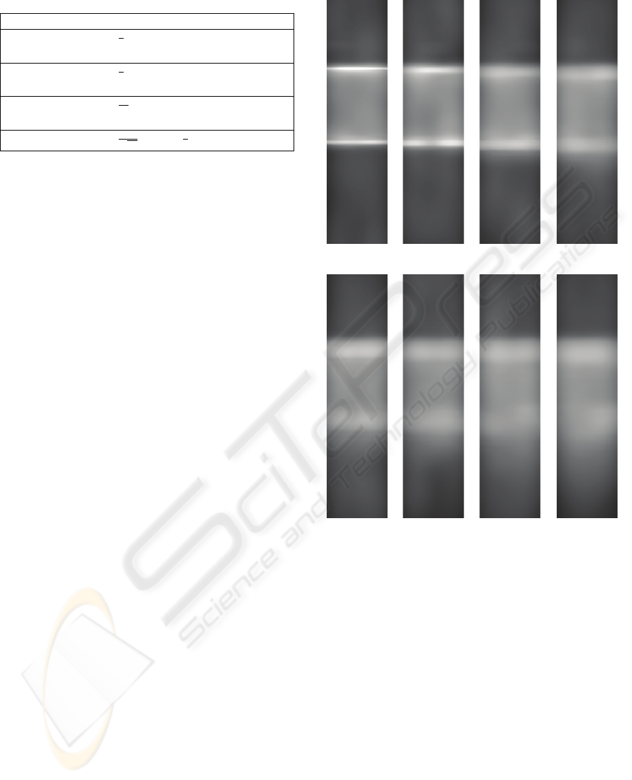
Table 2: Univariate kernel functions.

Kernel K

(y)

Uniform

if y < 1,

0 otherwise

Epanechnikov

(1 −y) if y < 1,

0 otherwise

Biweight

(1 −y)

if y < 1,

0 otherwise

Gaussian

√

2π

exp



−



such that the light form caustics on a plane beneath

the wave. A virtual camera is placed such that the

caustics are clearly visible.

We have rendered the scene using temporal pho-

ton differentials, and Cammarano and Jensen’s time

dependent photon mapping. The images in Figure 5

are renderings of the same frame but at different expo-

sures, e. They were rendered using temporal photon

differentials and a photon map containing only 1000

photons. From the images we notice that the tempo-

ral photon differentials assume the expected behavior.

As the exposure increases the caustics are blurred ac-

quiring a comets tail away from the direction of move-

ment. This is the behavior chosen at implementation

time. We could just as well have placed the time de-

pendent kernel centered over the photon intersection

point and likewise have centered the time ﬁltering or

we could just have centered the ﬁltering. As it is, the

time differential is ’trailing’ after the photon both in

respect to placement and ﬁltering. As we shall see,

though it is hardly visible, the same strategy has been

implemented for time dependent photon mapping.

The renderings in Figure 6 have all except (a) been

created with time dependent photon mapping. Addi-

tionally, all images were rendered using the same ex-

posure, e = 1.0 frame. Figure 6(a) has been included

for comparison, it was rendered using temporal pho-

ton differentials and is a copy of the image in Figure 5

with an exposure 1.0 frame. First of all, what we see

from Figure 6(b) is that the bias versus variance trade-

off provided by time dependent photon mapping is

too poor to produce palpable caustics. For this rea-

son a much higher number photons have been used

to render the images in the three rightmost columns.

Of these, the top row is based on a photon map con-

taining as much as 480 000 photons while the bot-

tom row is based on a photon map contain 40 000

photons. From left to right the temporal resolution

increases from 0 to 2 to 10 in-between frames. The

spatial bandwidth for the renderings was chosen as

to decrease noise to an acceptable level. This leads

to the perhaps most important observation, namely

that a low temporal resolution produces visible bands

that can only be removed by ﬁltering beyond what re-

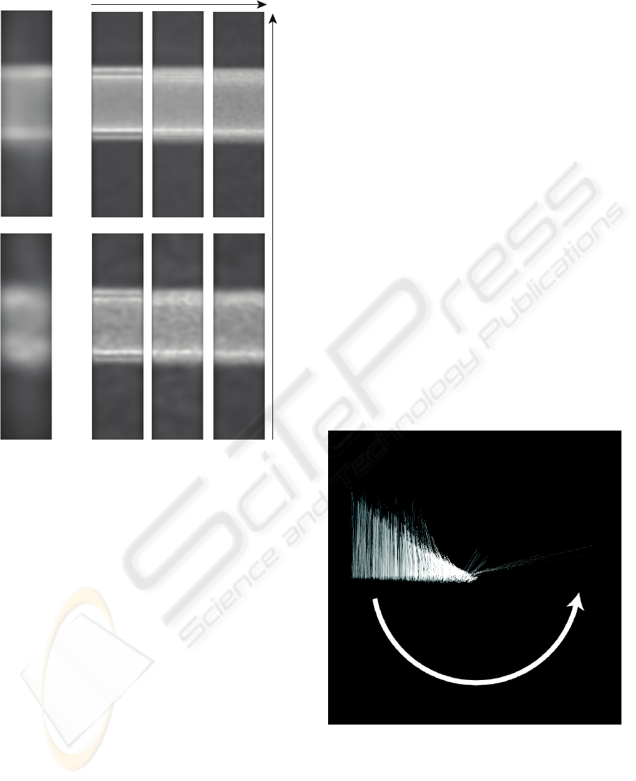
1/12 1/4 1/2 3/4

1 5/4 3/2 7/4

Figure 5: Renderings of the case study scene using tempo-

ral photon differentials. The number under the renderings

indicate exposure, e. All images are rendered at the same

frame step using a photon map containing 1 000 photons.

moves normal noise. This complicates matter, as an

increase of photons no longer is a guarantee for high

quality illumination.

Photon differentials are free of this concern as the

blurring is based on the ﬁrst order derivatives of object

movement and not on ﬁnite animation steps. In the

implementation presented here one additional frame

is need in order to estimate the derivatives.

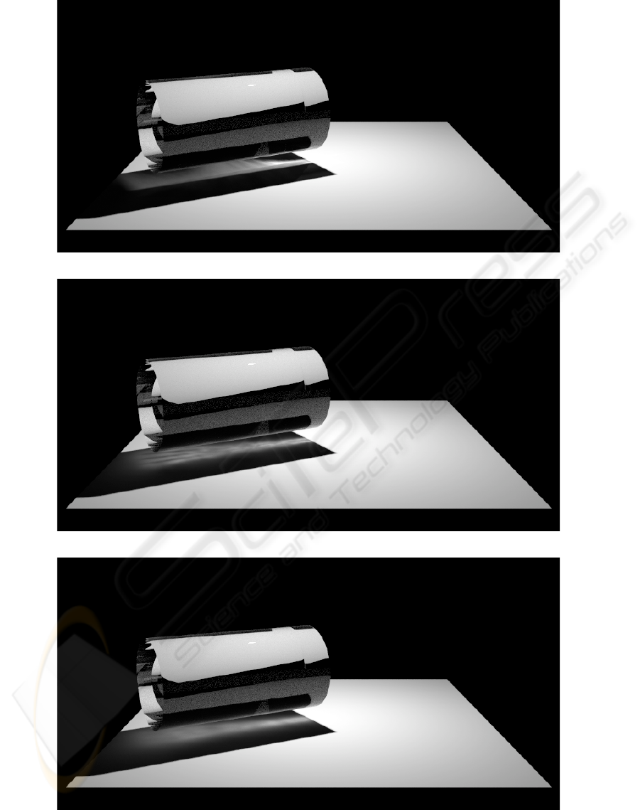
The images in Figure 7 present a more complex–

all though very artiﬁcial–scene, in which a cylinder

is rotating counterclockwise around its one end. This

rotation means that the speed of the cylinder will in-

crease as we move from the turning point down the

length of the cylinder. As a result the produced caustic

becomes more blurred when refracted from the high-

GRAPP 2010 - International Conference on Computer Graphics Theory and Applications

(a)

(b)

(c)

Figure 7: Rendering of a rotating cylinder. All images were render with a exposure of 1.0 frames, using a photon map

containing 5000 photons. Figure 7(a) was rendered using temporal photon differentials. Figures 7(b) and 7(c) were rendered

using time dependent photon mapping the former using 100 photons per radiance estimate and the latter using 250 photons in

the radiance estimate.

TEMPORAL PHOTON DIFFERENTIALS

resolution of photon map

temporal resolution

(f) (g) (h)

(a)

(b)

Figure 6: Comparing temporal photon differentials with

time dependent photon differentials. Rendering in (a)

shows temporal photon differentials using 1 000 photons,

(b) shows time dependent photon differentials using 1 000

photons, (c)-(e) shows time dependent photon differentials

using 480 000 photons with 0, 2, and 10 in-between frames

respectively, and (f)-(g) shows time dependent photon dif-

ferentials using 40 000 photons with 0, 2, and 10 in-between

frames respectively. The exposure for all images is 1.0

frame.

speed end of the cylinder. Figure 7(a) gives the solu-

tion provided by temporal photon differentials while

the images in Figures 7(b) and 7(c) were produced

with time dependent photon mapping. All images

were rendered with the same number of photons con-

tained in the photon map. However, the two latter im-

ages were rendered with different bandwidths. From

these two images we see that at this obviously low

temporal resolution an increase in bandwidth can help

remove the temporal bands that time dependent pho-

ton mapping is prone to. The price, however, is an

unwanted blurring of the front of the caustic.

Finally, Figure 8 solely depicts the photons’ time

differentials as they are projected down on the plane

beneath the cylinder.

A high exposure time has been used as to facilitate

the illustration. The image conﬁrms that the time dif-

ferential vectors become longer when refracted from

the high-speed end of the cylinder, thus elongating the

time dependent kernel used in the temporal radiance

estimate.

4 CONCLUSIONS

In this paper we have presented temporal photon dif-

ferentials – a global illumination method for render-

ing animated scenes. Temporal photon differentials

elegantly handles time ﬁltering such that frames can

be rendered on a one to one basis. Since velocity

is a relative concept, out method handles camera as

well as object motion, further in contrast to simi-

lar dynamic scene renderer, temporal photon differ-

entials does not need in-between frames in order to

avoid temporal aliasing. Finally, temporal photon dif-

ferentials includes photon differential’s ability to ef-

ﬁciently and sharply model caustics in still frames,

and it further improves the computationally efﬁciency

for animations by reusing photons from earlier frames

through the ﬁrst order spatial-temporal model of pho-

ton incidence.

Figure 8: Projected time differentials from a rotating glass

cylinder.

GRAPP 2010 - International Conference on Computer Graphics Theory and Applications

REFERENCES

Cammarano, M. and Jensen, H. W. (2002). Time depen-

dent photon mapping. In EGRW ’02: Proceedings of

the 13th Eurographics workshop on Rendering, pages

135–144, Aire-la-Ville, Switzerland, Switzerland. Eu-

rographics Association.

Christensen, P. H., Laur, D. M., Fong, J., Wooten, W. L.,

and Batali, D. (2003). Ray differentials and multires-

olution geometry caching for distribution ray tracing

in complex scenes. In Proceedings of Eurograph-

ics 2003, Computer Graphics Forum, pages 543–552.

Blackwell Publishing Inc.

Cook, R. L., Porter, T., and Carpenter, L. (1984). Dis-

tributed ray tracing. SIGGRAPH Comput. Graphics,

18(3):137–145.

Durand, F., Holzschuch, N., Soler, C., Chan, E., and Sillion,

F. X. (2005). A frequency analysis of light transport.

In Marks, J., editor, ACM SIGGRAPH 2005, pages

1115–1126.

Egan, K., Tseng, Y.-T., Holzschuch, N., Durand, F.,

and Ramamoorthi, R. (2009). Frequency Analysis

and Sheared Reconstruction for Rendering Motion

Blur. SIGGRAPH (ACM Transactions on Graphics),

28(3):93:1–93:13.

Gjøl, M., Larsen, B. D., and Christensen, N.-J. (2008). Final

gathering using ray differentials. In Proceedings of

WSCG 2008, pages 41–46.

Haeberli, P. and Akeley, K. (1990). The accumulation

buffer: hardware support for high-quality rendering.

In SIGGRAPH ’90: Proceedings of the 17th an-

nual conference on Computer graphics and interac-

tive techniques, pages 309–318, New York, NY, USA.

ACM.

Igehy, H. (1999). Tracing ray differential. In Rockwood, A.,

editor, Siggraph 1999, Computer Graphics Proceed-

ings, pages 179–186, Los Angeles. Addison Wesley

Longman.

Myszkowski, K., Tawara, T., Akamine, H., and Seidel, H.-

P. (2001). Perception-guided global illumination solu-

tion for animation rendering. In SIGGRAPH ’01: Pro-

ceedings of the 28th annual conference on Computer

graphics and interactive techniques, pages 221–230,

New York, NY, USA. ACM.

Schjøth, L., Frisvad, J. R., Erleben, K., and Sporring, J.

(2007). Photon differentials. In GRAPHITE ’07: Pro-

ceedings of the 5th international conference on Com-

puter graphics and interactive techniques in Australia

and Southeast Asia, pages 179–186, New York, NY,

USA. ACM.

Sporring, J., Schjøth, L., and Erleben, K. (2009). Spa-

tial and Temporal Ray Differentials. Technical Re-

port 09/04, Institute of Computer Science, University

of Copenhagen, Copenhagen, Denmark. ISSN: 0107-

8283.

Tawara, T., Myszkowski, K., Dmitriev, K., Havran, V.,

Damez, C., and Seidel, H.-P. (2004). Exploiting tem-

poral coherence in global illumination. In SCCG ’04:

Proceedings of the 20th spring conference on Com-

puter graphics, pages 23–33, New York, NY, USA.

ACM.

TEMPORAL PHOTON DIFFERENTIALS