A NEW APPROACH FOR DETECTING LOCAL FEATURES
Giang Phuong Nguyen and Hans Jørgen Andersen
Department of Media Technology, Aalborg University, Denmark
Keywords:
Local descriptors, Image features, Triangular representation, Image retrieval/recognition.
Abstract:
Local features up to now are often mentioned in the meaning of interest points. A patch around each point
is formed to compute descriptors or feature vectors. Therefore, in order to satisfy different invariant imaging
conditions such as scales and viewpoints, an input image is often represented in a scale-space, i.e. size of
patches are defined by their corresponding scales. Our proposed technique for detecting local features is
different, where no scale-space is required, by dividing the given image into a number of triangles with sizes
dependent on the content of the image at the location of each triangle. In this paper, we demonstrate that the
triangular representation of images provide invariant features of the image. Experiments using these features
show higher retrieval performance over existing methods.
1 INTRODUCTION
At the beginning of image retrieval systems, global
features such as color histograms were commonly
used. Recently, local features is taking the role.
There are several advantages of local features over
global features including robustness to occlusion and
clutter, distinctiveness for differentiating in a large
set of objects, a large quantity can be extracted in
a single image, and invariant to translation, rotation
etc. These advantages lead to the increasing num-
ber of researches on exploring these types of features.
Comprehensive overviews can be found in (Mikola-
jczyk and Schmid, 2005; Tuytelaars and Mikolajczyk,
2008).
Up to now, local features is mostly known as
descriptors extracted from areas located at interest
points (Tuytelaars and Mikolajczyk, 2008). This
means that, existing methods first detect interest
points, for example using Harris corner detector (Har-
ris and Stephens, 1988). Then a patch is drawn which
is centered at the corresponding interest point, and
descriptors are computed from each patch. So, the
main issue is how to define the size of the patch.
In other words, how to make these descriptors scale
invariant. To satisfy this requirement, these meth-
ods need to locate a given image at different scales,
or so called the scale-space approach. A given im-
age is represented in a scale-space using difference
of Gaussian and down sampling (Lowe, 2004; Brown
and Lowe, 2007; Nguyen and Andersen, 2008). The
size of a patch depends on the corresponding scale
where the interest point is detected. The computation
of the scale space and descriptors is often expensive
and complicated.
In this paper, we propose a different approach
for detecting local features that does not require the
scale-space representation nor the detection of inter-
est points. Given an input image, we divide the image
into a number of right triangles where a triangle de-
fines a homogenous region. The size of each triangle
depends on the content of the image at the location of
the triangle. This process is done automatically. This
means that if an object appears at different scales, the
triangular representation will adapt to draw the corre-
sponding triangle size. The technique of using trian-
gle representation of images is originally introduced
by Distasi in (Distasi et al., 1997) for image com-
pression. Moreover, in this reference, only intensity
images are taken into account. Following the current
trend, where color based local features are of inter-
est, we also investigate the use of color information
for describing local features. The distinctiveness in
color is much larger, therefore, using color informa-
tion for locating local features can be of great impor-
tance when matching images. We develop a new tech-
nique to extract local features using the color based
triangular representation of images.
The paper is organized as follows. In the next sec-
tion, we will give a description of our approach in
using triangular representation of color images, and
how to compute local descriptors. In section 2.4, we
221
Phuong Nguyen G. and Jørgen Andersen H. (2010).
A NEW APPROACH FOR DETECTING LOCAL FEATURES.
In Proceedings of the International Conference on Computer Vision Theory and Applications, pages 221-226
DOI: 10.5220/0002848402210226
Copyright
c
 SciTePress

evaluate the proposed features with repeatability cri-
teria in (Mikolajczyk and Schmid, 2005). Experimen-
tal results in a image retrieval system are carried out
in section 3.
2 BTREE TRIANGULAR CODING
(BTTC) FOR COLOR IMAGE
In this section, we discuss the extension of the trian-
gular representation for intensity images to color im-
ages. We then evaluate the repeatability of our local
features under different imaging conditions.
2.1 1D-BTTC
As mentioned above, the BTree triangular coding
(BTTC) is a method originally designed for image
compression purpose (Distasi et al., 1997). An input
image is an intensity image, so we denote it as 1D-
BTTC. For compression purpose, the method tries to
find a set of pixels from a given image that is able to
represent the content of the whole image. This means
that given a set of pixels, the rest of pixels can be in-
terpolated using this set. In the reference, the authors
divide an image into a number of triangles, where pix-
els within a triangle can be interpolated using infor-
mation of the three vertices. The same idea can be
applied to segment an image into a number of local
areas, where each area is a homogenous triangle.
Figure 1: An illustration of building BTree using BTTC.
The last figure shows an example of a final BTree.
A given image I is considered as a finite set of
points in a 3-dimensional space, i.e. I = {(x, y, c)|c =
F(x, y)} where (x, y) denotes pixel position, and c is
an intensity value. BTTC tries to approximate I with
a discrete surface B = {(x , y, d)|d = G(x, y)}, defined
by a finite set of polyhedrons. In this case, a poly-
hedron is a right-angled triangle (RAT). Assuming a
RAT with three vertices (x
1
, y
1
), (x
2
, y
2
), (x
3
, y
3
) and
c
1
= F(x
1
, y
1
), c
2
= F(x
2
, y
2
), c
3
= F(x
3
, y
3
), we have
a set {x
i
, y
i
, c
i
}
i=1..3
∈ I. The approximating function
G(x, y) is computed by linear interpolation:
G(x, y) = c
1
+ α(c
2
−c
1
) + β(c
3
−c
1
) (1)
where α and β are defined by the two relations:
α =
(x −x
1
)(y
3
−y
1
) −(y −y
1
)(x
3
−x
1
)
(x
2
−x
1
)(y
3
−y
1
) −(y
2
−y
1
)(x
3
−x
1
)
(2)
β =
(x
2
−x
1
)(y −y
1
) −(y
2
−y
1
)(x −x
1
)
(x
2
−x
1
)(y
3
−y
1
) −(y
2
−y
1
)(x
3
−x
1
)
(3)
An error function is used to check the approximation:
err = |F(x, y) −G(x, y)| ≤ ε, ε > 0 (4)
If the above condition is not met then the tri-
angle is divided along its height relative to the hy-
potenuse, replacing itself with two new RATs. The
coding scheme runs recursively until no more division
takes place. In the worst case, the process is stopped
when it reaches to the pixel level i.e. three vertices
of a RAT are three neighbor pixels and err=0. The
decomposition is arranged in a binary tree. Without
loss of generality, the given image is assumed hav-
ing square shape, otherwise the image is padded in a
suitable way. With this assumption, all RAT will be
isosceles. Finally, all points at the leave level are used
for the compression process. Figure 1 shows an illus-
tration of the above process.
In the reference (Distasi et al., 1997), experi-
ments prove that BTTC produces images of satisfac-
tory quality in objective and subjective point of view.
Furthermore, this method has shown very fast in ex-
ecution time, which is also an essential factor in any
processing system. We note here that for encoding
purpose, the number of points (or RAT) is very high
(up to several ten thousand vertices depending on the
image content). However, we do not need that detail
level, so by increasing the error threshold in Eq.(4)
larger we obtain fewer RATs while still fulfilling the
homogenous region criteria. Examples using BTTC
to represent image content with different threshold
values are shown in figure 2.
2.2 3D-BTTC
In this section, we extend the 1D-BTTC to color im-
age. As we mentioned above, the use of color infor-
mation can be of great importance for matching im-
ages. To get a triangular representation on the color
image, we consider the 3-color channels at the same
time, so the technique is called 3D-BTTC.
VISAPP 2010 - International Conference on Computer Vision Theory and Applications
222

(a) (b)
(c) (d)
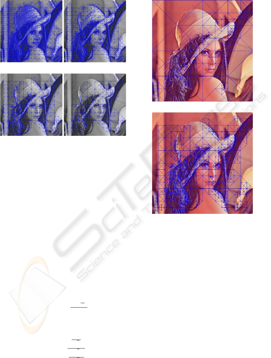
Figure 2: Examples using 1D-BTTC embedded in the input
image: with different values of the threshold, the higher the
threshold, the rougher the triangular representation.
First of all, we consider the color space of the
given image. Because of common variations in
imaging conditions such as shading, shadows, or re-
flectance, the components of the RGB color space are
correlated and very sensitive to illumination changes.
Therefore, different color spaces are investigated, for
instance, normalized RGB, HSI, or Lab. There are
several comprehensive overviews on characteristics
of existing color spaces (Niblack, 1985; Gevers et al.,
2006; Geusbroek et al., 2001; Gevers and Smeulders,
1999), where each color system is evaluated under
different invariant criteria. HSI (Hue, Saturation and
Intensity) is among one of the best color space that
overcomes shading, shadows, reflectance, and only
color differences are taken into account. We, there-
fore, convert all input images into the HSI color space.
Given an RGB image, the HSI color space is com-
puted by the following equation:


H
S
I


=



tan
−1
(
o
1
o
2
)
q
o
2
1
+ o
2
2
o
3



, (5)
where


o
1
o
2
o
3


=



R−G
√
2
R+G−2B
√
6
R+G+B
√
3



. (6)
(a)
(b)
Figure 3: An example of triangular representation using 1D-
BTTC (a) and 3D-BTTC (b) embedded to the input image.
An input image I is now represented as I = {(x, y, c)}
where (x, y) denotes pixel position, and c = {H, S, I}.
Similar to 1D-BTTC, the HSI image is first divided
into two triangles along the diagonal of the given im-
age. The condition in Eq.(4) must be satisfied for all
three channels. This means that for each pixel within
a triangle, we compute the interpolated color based on
the color of the three vertices. Eq.(1) is extended as:
G
H
(x, y) = H
1
+ α(H
2
−H
1
) + β(H
3
−H
1
) (7)
G
S
(x, y) = S
1
+ α(S
2
−S
1
) + β(S
3
−S
1
) (8)
G
I
(x, y) = I
1
+ α(I
2
−I
1
) + β(I
3
−I
1
) (9)
where α and β are computed by Eq.(2). H
i
, S
i
and
I
i
(i = 1, 2, 3) are HSI values of the three vertices of
the current triangle. For 3D-BTTC, Eq.(4) changes as
follows
A NEW APPROACH FOR DETECTING LOCAL FEATURES
223

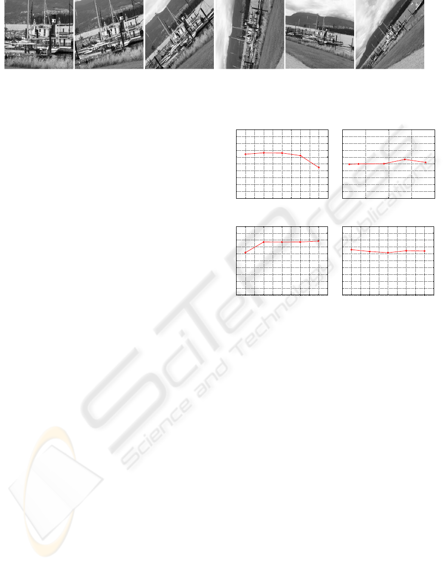
Figure 4: The ”boat” test set for evaluating the repeatability when changing rotations and scales.
|F
H
(x, y) −G
H
(x, y)| ≤ε
H
, ε
H
> 0 (10)
|F
S
(x, y) −G
S
(x, y)| ≤ ε
S
, ε
S
> 0 (11)
|F
I
(x, y) −G
I
(x, y)| ≤ ε
I
, ε
I
> 0 (12)
If all the color channels meet the above equations,
then the division stops, otherwise two new triangles
are created. The process is repeated, the stopping cri-
teria is similar to the 1D-BTTC.
In figure 3, we show an example of using 1D-
BTTC and 3D-BTTC. The input image is converted
to an intensity image and a HSI image, respectively.
The threshold are set equal in both cases. We can ob-
serve that there are a lot interesting area where color
changes and they are ignored when using 1D-BTTC,
but captured in case of 3D-BTTC.
2.3 Computing Descriptors
When the triangular representation of the given image
are drawn, we calculate the HSI color histogram of
each right triangle. The color histogram is used as
descriptor of the triangle.
2.4 Repeatability Experiment
In this section, we evaluate the repeatability of our lo-
cal features. In (Mikolajczyk et al., 2005), the authors
suggest a test for the quality of local features under
different challenges. Each challenge contains of a set
of 6 images with a reference image and 5 other im-
ages show the same scene under predefined changes
including blurring, rotation, zooming, viewpoint, and
lighting. Figure 4 shows an example of a set with dif-
ferent rotations and scales.
The repeatability rate is defined as the ratio be-
tween the number of actual corresponding features
and the total number of features that occur in the area
common to both images. To compute the rate, local
features are extracted from all test images. Then, fea-
tures from the reference image will be mapped to each
images of the other five images using a predefined
transformation matrix (Mikolajczyk et al., 2005). All
features outside the common area between two im-
ages are removed. After that, we calculate the overlap
between features from the reference image to features
of the other images. Similar to (Mikolajczyk et al.,
2005), we also set the overlap error threshold to 40%.
15 20 25 30 35 40 45 50 55 60 65
0
10
20
30
40
50
60
70
80
90
100
viewpoint angle
repeatability %
(a)
1 1.5 2 2.5 3
0
10
20
30
40
50
60
70
80
90
100
scale changes
repeatability %
(b)
1.5 2 2.5 3 3.5 4 4.5 5 5.5 6 6.5
0
10
20
30
40
50
60
70
80
90
100
increasing blur
repeatability %
(c)
1.5 2 2.5 3 3.5 4 4.5 5 5.5 6 6.5
0
10
20
30
40
50
60
70
80
90
100
decreasing light
repeatability %
(d)
Figure 5: Repeatability of 3D-BTTC under different imag-
ing conditions. (a) With different viewpoint angles. (b)
With different scales (including zooming and rotation). (c)
With different blurring factors. (d) With different illumina-
tion.
In figure 5, we show results with four different test
sets corresponding to four different challenges: view-
point changes, scale changes, increasing blurring, and
decreasing lighting. Results show that our local fea-
tures give very stable repeatability rate in different
imaging conditions. For examples, with viewpoints
changes of 40
0
to the reference image, the repeata-
bility rate is 65%, this is compatible to methods pre-
sented in (Mikolajczyk et al., 2005). In case of rota-
tion and zooming applied, our local features is stable
even with large scale changes. In (Mikolajczyk et al.,
2005), other methods go down quite significantly with
larger scales. In this reference, the best performance
reaches 30% rate at the highest scale, and our method
stays at 50% rate. Given very high challenging test
sets, on average, we obtain 60% repeatability rate for
all cases.
VISAPP 2010 - International Conference on Computer Vision Theory and Applications
224

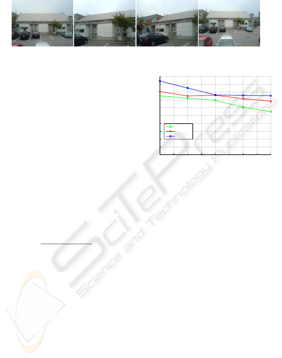
Figure 6: An example of images taken from the same building.
3 EXPERIMENTAL RESULTS
Our experiments are carried out with a dataset, which
contains of 135 images. This dataset is called the
AAU dataset, where images are captured from 21
buildings/objects in the area of Aalborg University.
There are from 4 to 7 images for each building. It
should be noted that all the buildings are quite similar
in their textures (for examples, brick wall or glasses).
Images of the same building are taken at different
viewpoints, rotations, and scales. In figure 6, we show
example images of the same building.
Evaluation of local features is based on image re-
trieval performance. To do so, we sequentially use
images from the given dataset as a query image. Lo-
cal features are extracted from the query image and
compared to features of all images in the dataset. The
ε
i
(i = 1, 2, 3) in Eq.(10) are all set to 150. For com-
paring HSI histograms, we use the Euclidean distance
as a similarity function. The top 5 best matching are
returned, and groundtruth is manually assigned to cor-
responding building to compute the precision rate:
precision =
# of correct matches
# of returned images
(%). (13)
The average retrieval rate is shown in figure 7.
We also reported the retrieval performance using the
multi-scale oriented patches (MOPS) (Brown et al.,
2005), which applies the common approach using
scale-space representation, for comparison. Match-
ing using 1D-BTTC also used as a reference. Results
show that using color information instead of intensity
boot up the retrieval performance. Moreover, our sys-
tem using 3D-BTTC give a higher retrieval rate com-
pared to MOPS.
4 CONCLUSIONS
In this paper, we present a new approach to detect lo-
cal features in color images. We use triangular rep-
resentation to detect local features. Depends on the
content of the area inside the input image, different
sizes of triangles are drawn. Therefore, our proposed
1 1.5 2 2.5 3 3.5 4 4.5 5
0
10
20
30
40
50
60
70
80
90
100
Matching performance on top 5 images
number of images
average precision (%)
1D−BTTC
MOPS
3D−BTTC
Figure 7: Precision vs. number of returned images.
approach is independent of changing scales without
using the scale-space representation. The technique is
much simpler and, hence, faster. Besides, the repeata-
bility rate of our local features in different imaging
conditions is compatible to existing techniques. Our
first experimental results on image retrieval show that
the proposed approach gives better performance com-
pared to other method using scale-space representa-
tion. We obtain a high precision rate, i.e. 95% correct
matches in the best matching results.
ACKNOWLEDGEMENTS
This research is supported by the IPCity project (FP-
2004-IST-4-27571), a EU-funded Sixth Framework
program Integrated project on Interaction and Pres-
ence in Urban Environments.
REFERENCES
Brown, M. and Lowe, D. (2007). Automatic panoramic im-
age stitching using invariant features. International
Journal of Computer Vision, 74(1):59–73.
Brown, M., Szeliski, R., and Winder, S. (2005). Multi-
image matching using multi-scale oriented patches. In
Proceedings of the IEEE Conference on Computer Vi-
sion and Pattern Recognition, volume 1, pages 510–
517.
A NEW APPROACH FOR DETECTING LOCAL FEATURES
225

Distasi, R., Nappi, M., and Vitulano, S. (1997). Image com-
pression by B-Tree triangular coding. IEEE Transac-
tions on Communications, 45(9):1095–1100.
Geusbroek, J., Boomgaard, R., and Smeulders, A. (2001).
Color invariance. IEEE Transactions on Pattern Anal-
ysis and Machine Intelligence, 23(12):1338–1350.
Gevers, T. and Smeulders, A. (1999). Color based object
recognition. Pattern Recognition, 32:453–464.
Gevers, T., Weijer, J., and Stokman, H. (2006). Color fea-
ture detection. Color Image Processing: Methods and
Applications, editors R. Lukac and K.N. Plataniotis,
CRC Press.
Harris, C. and Stephens, M. (1988). A combined corner
and edge detector. Proceedings of the Alvey Vision
Conference, pages 147–151.
Lowe, D. (2004). Distinctive image features from scale-
invariant keypoints. International Journal of Com-
puter Vision, 60(2):91–110.
Mikolajczyk, K. and Schmid, C. (2005). A perfor-
mance evaluation of local descriptors. IEEE Trans-
actions on Pattern Analysis & Machine Intelligence,
27(10):1615–1630.
Mikolajczyk, K., Tuytelaars, T., Schmid, C., Zisserman, A.,
Matas, J., Schaffalitzky, F., Kadir, T., and Van-Gool,
L. (2005). A comparison of affine region detectors. In-
ternational Journal of Computer Vision, 1/2(65):43–
72.
Nguyen, G. and Andersen, H. (2008). Urban building
recognition during significant temporal variations. In
Proceedings of the IEEE Workshop on Applications of
Computer Vision, pages 1–6.
Niblack, W. (1985). An introduction to digital image pro-
cessing. Strandberg Publishing Company, Birkeroed,
Denmark, Denmark.
Tuytelaars, T. and Mikolajczyk, K. (2008). Local invariant
feature detectors. Foundations and Trends in Com-
puter Graphics and Vision, 3(3):177–280.
VISAPP 2010 - International Conference on Computer Vision Theory and Applications
226