COONS TRIANGULAR B
´
EZIER SURFACES
A. Arnal and A. Lluch
Dep. de Matem
`
atiques, Universitat Jaume I, Castell
´
o, Spain
Keywords:
Coons patches, Functional extremals, Triangular B
´
ezier surfaces, Masks.
Abstract:
In this paper we give some different surface generation methods starting out from prescribed boundary curves.
If the boundary control points are known it is natural to think of Coons patches, a popular solution of the prob-
lem of finding a surface given its boundary curves. We have developed three methods to generate triangular
patches given the boundary curves. First we give a discrete version of the triangular Coons patch. A second
method lets us to find the extremals of a functional as a solution of a linear system of the control points. That
functional is the one that minimizes the Coons patch. The third method makes it possible to build a B
´
ezier
triangle by means of a mask deduced from the characterization of cubical extremals of the functional.
1 INTRODUCTION
One of the oldest surface problems in CAGD is the
following: given the boundary curves, find the para-
metric surface
−→
x with these as boundary curves with
no other restriction. A popular solution of this prob-
lem is the Coons patch.
One of the aims of this paper is to find the ex-
tremals of a functional as a solution of a linear system
of the control points. This functional is the one that
minimizes the Coons patch.
Some other work about finding extremals of a
functional was already done. For rectangular patches
in (Monterde, 2003), (Monterde, 2004) and (Mon-
terde and Ugail, 2004), the functional they work with
is the Dirichlet functional. The Dirichlet functional
is related with the theory of minimal surfaces due to
the fact that is a linear functional having the same
extremals as the area functional. For the triangu-
lar B
´
ezier case (Arnal et al., 2003) worked with the
Dirichlet functional too. When the geometric prob-
lem is get B
´
ezier approximations to constant mean
curvature surfaces the study of the appropriate func-
tional appears in (Arnal et al., 2008). Finally, in a
more general way, for rectangular patches in (Mon-
terde and Ugail, 2006) a general quadratic functional
was studied.
Before we present our study about triangular
Coons patches, let us describe the more conventional
rectangular Coons patch and its properties.
2 BACKGROUND ON COONS
RECTANGULAR PATCHES
Coons first described this type of interpolant in
(Coons, 1967). It is assumed that four boundary
curves are given, which it is convenient to think of
as coming from a surface denoted
−→
x
0
, and so the nota-
tion
−→
x
0
(u, 0),
−→
x
0
(u, 1),
−→
x
0
(0, v) and
−→
x
0
(1, v) is used
to represent these boundary curves. The bilinearly
blended Coons patch that interpolates to the given
boundary curves is defined by:
−→
x (u, v) = (1− u)
−→
x
0
(0, v) + u
−→
x
0
(1, v)
+ (1− v)
−→
x
0
(u, 0) + v
−→
x
0
(u, 1)
−

1− u u


−→
x
0
(0, 0)
−→
x
0
(0, 1)
−→
x
0
(1, 0)
−→
x
0
(1, 1)

1− v
v

.
The Coons rectangular patch interpolates four bound-
ary curves and in addition is an extremal of the func-
tional
F (
−→
x ) =
Z
U
k
−→
x
uv
k
2
dudv, (1)
where U = [0, 1] × [0, 1], over all patches,
−→
x ∈
C
∞
[u, v], with a prescribed boundary. The Coons
patch was described in (Nielson et al., 1978) as
the unique interpolant that minimizes the functional
F (
−→
x ).
In general if a surface,
−→
x , is an extremal of a func-
tional, then it satisfies the associated Euler-Lagrange
equation, which, for this functional, is the PDE
148
Arnal A. and Lluch A. (2010).
COONS TRIANGULAR BÉZIER SURFACES.
In Proceedings of the International Conference on Computer Graphics Theory and Applications, pages 148-153
DOI: 10.5220/0002848601480153
Copyright
c
 SciTePress

−→
x
uuvv
= 0. (2)
Therefore the Coons patch can be considered as
a PDE surface, since it is a solution of the equation
above.
Instead of working with the general problem of
finding extremals of the functional F , we will con-
sider a restricted problem, namely that of finding
the polynomial patch that minimizes the functional
among all polynomial patches with the same bound-
ary.
Some work related with rectangular Coons
patches was carried out in (Farin and Hansford,
1999). While the boundary curves
−→
x
0
(u, 0),
−→
x
0
(u, 1),
−→
x
0
(0, v) and
−→
x
0
(1, v) may be totally arbitrary, in the
early days the boundary curves were considered as
discretized curves with many points on them. In fact,
in (Farin and Hansford, 1999) these boundary poly-
gons are treated as B
´
ezier border control points and a
discrete version of the Coons patch is given. The inte-
rior control points P
i, j
are defined in terms of bound-
ary points by the discrete Coons patch:
P
i, j
=

1−
i
m

P
0, j
+
i
m
P
m, j
+

1−
j
m

P
i,0
+
j
n
P
i,n
−

1−
i
m
i
m


P
0,0
P
0,n
P
m,0
P
m,n

1−
j
n
j
n

.
for 0 < i < m and 0 < j < n. These control points de-
fine the discrete Coons patch which is the same patch
as if Coons interpolation was applied to the B
´
ezier
curves associated to the boundary polygons.
The discrete Coons patch also minimizes the dis-
crete version of the functional F . In fact, the discrete
Coons patch is a PDE B
´
ezier surface satisfying the
discrete version of
−→
x
uuvv
= 0.
3 TRIANGULAR COONS
PATCHES
Now after introducing all these topics for rectangular
surfaces, let us come back to triangular patches. The
triangular Coons patch we will define first appeared
in (Nielson et al., 1978). Similar to the rectangular
Coons patch we consider the border curves
−→
x
0
(u, 0),
−→
x
0
(0, v) and
−→
x
0
(u, 1− u), (or
−→
x
0
(1− v, v)), to denote
the boundary curves and define the patch as
−→
x (u, v) =(1− u− v) (
−→
x
0
(u, 0) +
−→
x
0
(0, v) −
−→
x
0
(0, 0))
+ v(
−→
x
0
(0, u+ v) +
−→
x
0
(u, 1− u) −
−→
x
0
(0, 1))
+ u(
−→
x
0
(u+ v, 0) +
−→
x
0
(1− v, v) −
−→
x
0
(1, 0)).
x(0,v)
x(u,1-u)
x(u,0)
Figure 1: A representation of a triangular Coons patch.
Some differences with respect to the rectangular
Coons patch must be pointed out. First let us remark
that if we consider the border curves to be polyno-
mial curves of degree n, then the associated triangu-
lar Coons patch is a degree n+ 1 polynomial surface.
This increase in degree does not happen in the rectan-
gular case.
In contrast to the rectangular case we find two
more differences. First since the triangular patch is
not linear in both variables, then
−→
x
uuvv
6= 0. On the
other hand the Triangular Coons patch is not an ex-
tremal of the functional F . It can be proved that for
the triangular case, being an extremal of such a func-
tional is not equivalent to satisfying the associated
Euler-Lagrange equation, as was true for the rectan-
gular Coons patch: An extremal of the functional,
described in Equation (4), would coincide with the
solution of its associated Euler-Lagrange equation,
−→
x
uuvv
= 0, only under certain conditions on the con-
trol points.
Now, analogously to what was done in (Farin and
Hansford, 1999) for rectangular patches, we have ob-
tained the discrete version of the triangular Coons
patch.
Definition 1. The interior points P
i, j,k
with i + j +
k = n+1, of the Triangular Discrete Coons patch are
defined by
P
i, j,k
=
k
n+ 1
(P
i,0,n−i
+ P
0, j,n− j
− P
0,0,n
)
+
j
n+ 1
(P
0,n−k,k
+ P
i,n−i,0
− P
0,n,0
)
+
i
n+ 1
(P
n−k,0,k
+ P
n− j, j,0
− P
n,0,0
).
(3)
The triangular B
´
ezier surface with the previous in-
terior control points coincides with the triangular
Coons patch that would be obtained from the B
´
ezier
curves associated to the boundary control points.
In the following proposition we give a formula to
express the functional of a B
´
ezier triangular patch,
F (
−→
x ) =
Z
T
k
−→
x
uv
k
2
dudv, (4)
defined now in the region T = {(u, v) ∈ R
2
: 0 ≤
COONS TRIANGULAR BÉZIER SURFACES
149

Figure 2: Three discrete triangular Coons patches.
u, 0 ≤ v, u + v ≤ 1}, in terms of the control points
P
I
=

x
1
I
, x
2
I
, x
3
I

, where I = (i, j,k).
Proposition 2. The functional, F (
−→
x ), of a triangu-
lar B
´
ezier surface can be expressed by the formula
F (
−→
x ) =
3
∑
a=1
∑
|I
0
|=n
∑
|I
1
|=n
C
I
0
I
1
x
a
I
0
x
a
I
1
(5)
where |I| = i+ j+ k, and with
C
I
0
I
1
=2n(2n− 1)

n
I
0

n
I
1


2n
I
0
+I
1

(
1
2

b
12
12
+ b
13
13
+ b
23
23
+ b
33
33

− b
13
12
− b
23
12
+ b
33
12
+ b
23
13
− b
33
13
− b
33
23
),
(6)
where the coefficients b
tl
rs
satisfy the symmetry relation
b
tl
rs
= b
tl
sr
= b
lt
rs
= b
lt
sr
, and are defined by
b
tl
rs
=













































I
r
0
I
s
0
I
t
1
I
r
1
+I
r
1
I
s
1
I
t
0
I
r
0
(I
r
0
+I
r
1
)(I
s
0
+I
s
1
)(I
t
0
+I
t
1
)(I
r
0
+I
r
1
−1)
r = l
I
r
0
I
s
0
I
t
1
(I
t
1
−1)+I
r
1
I
s
1
I
t
0
(I
t
0
−1)
(I
r
0
+I
r
1
)(I
s
0
+I
s
1
)(I
t
0
+I
t
1
)(I
t
0
+I
t
1
−1)
t = l
2I
r
0
I
s
0
I
r
1
I
r
1
(I
r
0
+I
r
1
)(I
r
0
+I
r
1
−1)(I
s
0
+I
s
1
)(I
s
0
+I
s
1
−1)
r = t, s = l
2I
r
0
(I
r
0
−1)I
t
1
(I
t
1
−1)
(I
r
0
+I
r
1
)(I
r
0
+I
r
1
−1)(I
t
0
+I
t
1
)(I
t
0
+I
t
1
−1)
r = s,t = l
I
r
0
I
s
0
I
r
1
(I
r
1
−1)+I
r
1
I
s
1
I
r
0
(I
r
0
−1)
(I
r
0
+I
r
1
)(I
s
0
+I
s
1
)(I
r
0
+I
r
1
−1)(I
t
0
+I
t
1
−2)
r = t = l
2I
r
0
(I
r
0
−1)I
r
1
(I
r
1
−1)
(I
r
0
+I
r
1
)(I
r
0
+I
r
1
−1)(I
r
0
+I
r
1
−2)(I
r
0
+I
r
1
−3)
r = s = t = l.
(7)
Proof: The functional F is a second-order func-
tional and, therefore, in order to obtain the coeffi-
cients C
I
0
I
1
we compute its second derivative, first
from Equation (5):
∂
2
F (
−→
x )
∂x
a
I
0
∂x
a
I
1
=
∂
2
∂x
a
I
0
∂x
a
I
1
3
∑
¯a=1
∑
|I|=n
∑
|J|=n
C
IJ
x
¯a
I
x
¯a
J
=
∂
∂x
a
I
1
∑
|J|=n
2C
I
0
J
x
a
J
= 2C
I
0
I
1
.
And now, we compute the first derivative from Equa-
tion (4):
∂F (
−→
x )
∂x
a
I
0
=
Z
T
∂
∂x
a
I
0
k
−→
x
uv
k
2
dudv
=
Z
T
2 <
∂
−→
x
uv
∂x
a
I
0
,
−→
x
uv
> dudv
=
Z
T
2 < (B
n
I
0
)
uv
,
−→
x
uv
> dudv,
Let us denote by e
1
= (1, 0, 0), e
2
= (0, 1, 0), e
3
=
(0, 0, 1). Then, the second derivative is given by:
∂
2
F (
−→
x )
∂x
a
I
0
∂x
a
I
1
= 2
Z
T
< (B
n
I
0
)
uv
,
∂
−→
x
uv
∂x
a
I
1
> dudv
=2
Z
T
< (B
n
I
0
)
uv
, (B
n
I
1
)
uv
> dudv
=2
Z
T
n
2
(n− 1
2
)

B
n
I
0
−e
1
−e
2
− B
n
I
0
−e
1
−e
3
−B
n
I
0
−e
2
−e
3
+ B
n
I
0
−2e
3

B
n
I
1
−e
1
−e
2
− B
n
I
1
−e
1
−e
3
− B
n
I
1
−e
2
−e
3
+ B
n
I
1
−2e
3

dudv
=2n(2n− 1)

n
I
0

n
I
1


2n
I
0
+I
1

(
1
2

b
12
12
+ b
13
13
+ b
23
23
+ b
33
33

−b
13
12
− b
23
12
+ b
33
12
+ b
23
13
− b
33
13
− b
33
23
),
where we have computed the integral of the Bernstein
polynomials with the formula:
Z
T
B
2n−2
I
0
+I
1
(u, v) dudv =
1
(3n− 2)(3n− 3)
,
and we have performed some simplifications like the
following:
Z
T
B
n−1
I
0
−e
1
−e
2
B
n−1
I
1
−e
1
−e
3
+ B
n−1
I
1
−e
1
−e
2
B
n−1
I
0
−e
1
−e
3
dudv
=
Z
T

n−2
I
0
−e
1
−e
2

n−2
I
1
−e
1
−e
3

+

n−2
I
1
−e
1
−e
2

n−2
I
0
−e
1
−e
3


2n−4
I
0
+I
1
−2e
1
−e
2
−e
3

·
B
2n−4
I
0
+I
1
−2e
1
−e
2
−e
3
dudv
=
2n(2n− 1)
n
2
(n− 1
2
)

n
I
0

n
I
1


2n
I
0
+I
1

I
1
0
I
2
0
I
1
1
I
3
1
+ I
1
0
I
3
0
I
1
1
I
2
1
(I
1
0
+ I
1
1
)(I
2
0
+ I
2
1
)(I
1
0
+ I
1
1
− 1)(I
3
0
+ I
3
1
)
=
2n(2n− 1)
n
2
(n− 1
2
)

n
I
0

n
I
1


2n
I
0
+I
1

b
13
12
.
Therefore
C
I
0
I
1
=2n(2n− 1)

n
I
0

n
I
1


2n
I
0
+I
1

(
1
2

b
12
12
+ b
13
13
+ b
23
23
+ b
33
33

−b
13
12
− b
23
12
+ b
33
12
+ b
23
13
− b
33
13
− b
33
23
)
GRAPP 2010 - International Conference on Computer Graphics Theory and Applications
150

where b
tl
rs
are defined in Equation (7) .

Let us remark that the formula we give in Equa-
tion (5) translates the functional, F , into a function
of the control points. This fact, will allow us to com-
pute compute the gradient of the functional F with
respect to the coordinates of a general control point
P
I
0
=

x
1
I
0
, x
2
I
0
, x
3
I
0

to obtain an extremal of the func-
tional among all B
´
ezier surfaces with the same border
as a solution of a linear system.
Proposition 3. A triangular control net, P =
{P
I
}
|I|=n
, is an extremal of the functional, F , among
all triangular B
´
ezier surfaces with a prescribed
boundary if and only if:
∑
|J|=n
C
I
0
J
P
J
= 0 for all |I
0
= (I
1
0
, I
2
0
, I
3
0
)| = n (8)
with I
1
0
, I
2
0
, I
3
0
> 0, where C
IJ
are the coefficients de-
fined in Equation (6).
Proof: The gradient of the functional with respect
to the coordinates of an interior control point P
I
0
=

x
1
I
0
, x
2
I
0
, x
3
I
0

is given by
∂F (
−→
x )
∂P
I
0
=
∂F (
−→
x )
∂x
1
I
0
,
∂F (
−→
x )
∂x
2
I
0
,
∂F (
−→
x )
∂x
3
I
0
!
=2
∑
|J|=n
C
I
0
J
x
1
J
,
∑
|J|=n
C
I
0
J
x
2
J
,
∑
|J|=n
C
I
0
J
x
3
J
!
=2
∑
|J|=n
C
I
0
J
P
J
.

Equivalently, a triangular control net, P =
{P
I
}
|I|=n
, is an extremal among all control nets with
prescribed border control points if and only if
0 =
∑
|I|=n

n
I


2n
I
0
+I

(
1
2

b
12
12
+ b
13
13
+ b
23
23
+ b
33
33

−b
13
12
− b
23
12
+ b
33
12
+ b
23
13
− b
33
13
− b
33
23
)P
I
for all |I
0
= (I
1
0
, I
2
0
, I
3
0
)| = n with I
1
0
, I
2
0
, I
3
0
> 0, with the
coefficients b
tl
rs
given in Equation (7).
4 COONS MASKS AND
TRIANGULAR PERMANENCE
PATCHES
In general a condition that relates some control points
can be written by means of a mask only if (consider-
ing a 3× 3 triangular grid),
P
i−1, j−1,k+2
P
i−1, j,k+1
P
i−1, j+1,k
P
i−1, j+2,k−1
P
i, j−1,k+1
P
i, j,k
P
i, j+1,k−1
P
i+1, j−1,k
P
i+1, j,k−1
P
i+2, j−1,k−1
this condition relates the points on the grid in such a
way, that the interior point can be expressed in terms
of the boundary control points. The mask is then con-
sidered to be a stencil for the central point.
Some previous work related to masks can be
found in (Farin and Hansford, 1999). The rectan-
gular Coons patch, as well as the associated discrete
Coons patch, satisfies a Permanence Principle: Let
two points (u
0
, v
0
) and (u
1
, v
1
) define a rectangle R
in the domain U of the Coons patch. The four bound-
aries of this subpatch will map onto four curves on the
Coons patch. The Coons patch for those four bound-
ary curves is the original Coons patch restricted to
the rectangle R.
Moreover, as we said before, the rectangular
Coons patch is a PDE surface satisfying
−→
x
uuvv
= 0
and the discrete version of this partial differential
equation is verified exactly by the discrete Coons
patch. Farin and Hansford, in the previously cited
paper, (Farin and Hansford, 1999), deduced the fol-
lowing rectangular mask from this discrete PDE.
P
i, j
=
1
4
×
−1 2 −1
2 ⋆ 2
−1 2 −1
In that work, the authors generalized it by defining
what they called permanence patches: A permanence
patch is obtained from a control net
P
i, j
=
α β α
β ⋆ β
α β α
with 4α+ 4β = 1.
This kind of mask suggests the possibility of dif-
ferent choices for α and β, so in this sense Farin
and Hansford, show how some choices of these val-
ues give different masks which are also the discrete
form of a PDE, as the discrete version of the Euler-
Lagrange PDE
−→
x
uuvv
= 0, gave the first rectangular
mask α =
−1
4
.
Moreover Farin and Hansford extended the per-
manence patches concept to the triangular case just
by considering the analogous triangular mask.
Given a mask of the form
P
i, j,k
=
α β β α
β ⋆ β
β β
α
(9)
COONS TRIANGULAR BÉZIER SURFACES
151

with 3α + 6β = 1 the triangular patch formed with
such a control net is called a triangular permanence
patch.
Now, let us come back to rectangular patches and
show how the α =
−1
4
mask was deduced from the
Euler-Lagrange PDE
−→
x
uuvv
= 0.
The discrete version of
−→
x
uuvv
= 0 is given by
∆
2,2
P
i, j
= 0, where
∆
1,0
P
i, j
= P
i+1, j
− P
i, j
∆
0,1
P
i, j
= P
i, j+1
− P
i, j
.
Then
0 = ∆
2,2
P
i, j
= P
i+2, j+2
− 2P
i+2, j+1
− 2P
i+1, j+2
+4P
i+1, j+1
− 2P
i+1, j
− 2P
i, j+1
+ P
i+2, j
+ P
i, j+2
+ P
i, j
gives
P
i, j
=
−1
4
(P
i+1, j+1
− 2P
i+1, j
− 2P
i, j+1
− 2P
i, j−1
−2P
i−1, j
+ P
i+1, j−1
+ P
i−1, j+1
+ P
i−1, j−1
)
(10)
that is the rectangular mask α =
−1
4
.
This mask could also be deduced as a consequence
of the permanence principle. Let us show this. We
will determine for which value of α and β, with 4α +
4β = 1, a permanence patch satisfies the permanence
principle.
This principle implies that the control point P
i, j
can be obtained with the discrete Coons formula,
Equation (2), from the boundary control points on a
n × m grid or instead one can apply this formula to
any 3× 3 grid included in the global grid,
P
i−1, j−1
P
i−1, j
P
i−1, j+1
P
i, j−1
P
i, j
P
i, j+1
P
i+1, j−1
P
i+1, j
P
i+1, j+1
.
Therefore if we consider that any point in the
equation
P
i, j
=α(P
i+1, j+1
+ P
i+1, j−1
+ P
i−1, j−1
+ P
i−1, j+1
)
+β(P
i+1, j
+ P
i, j+1
+ P
i, j−1
+ P
i−1, j
),
can be written in terms of the boundary control points,
as we said by means of Equation (2), it leads us to the
value α =
−1
4
.
The permanence principle is not verified by trian-
gular Coons patches so the previous reasoning cannot
be followed in order to obtain a mask describing the
Coons triangle. Anyway we will introduce a mask,
which generates a permanence patch, since it is of the
kind defined in Equation (9), and which is related to
the triangular Coons patch.
We will consider the triangular control net of a tri-
angular Coons patch of degree 3, instead of the gen-
eral case of degree n,
P
003
P
012
P
021
P
030
P
102
P
111
P
120
P
201
P
210
P
300
The interior control point, P
111
, is defined, by Equa-
tion (3), in terms of the boundary control points of
a grid of degree 2. Moreover, the boundary con-
trol points on the degree 3 control net are the con-
trol points of the degree elevation of degree 2 border
curves.
To obtain a triangular mask grenerating a perma-
nence patch we will use the following result that gives
us a version of Proposition 3 for the case n = 3.
Proposition 4. A triangular control net of degree 3,
P = {P
I
}
|I|=3
, is an extremal of the functional, F (P ),
among all triangular control nets with a prescribed
boundary if and only if
P
111
=
1
2
(P
012
− P
021
+ P
102
+ P
120
− P
201
+ P
210
).
From this condition, given the exterior control
points in the case of degree n, we can generate the
whole triangular net by solving a linear system where
the equations are:
2P
i, j,k
= P
i−1, j,k+1
− P
i−1, j+1,k
+ P
i, j−1,k+1
+P
i, j+1,k−1
− P
i+1, j−1,k
+ P
i+1, j,k−1
P
i, j,k
being a interior control point. This equation can
be expressed by the following mask:
P
i, j,k
=
1
2
×
0 1 −1 0
1 ⋆ 1
−1 1
0
(11)
Then if we consider that any interior or border
control point in the equation
P
111
= α(P
003
+ P
030
+ P
300
)
+ β(P
012
+ P
021
+ P
102
+ P
201
+ P
120
+ P
210
)
can be written, thanks to Equation (3), in terms of
control points of a degree 2 control net, we find that
equality is only attained for the values α =
−2
3
and
β =
1
2
.
GRAPP 2010 - International Conference on Computer Graphics Theory and Applications
152

Therefore the triangular permanence patch for
α =
−2
3
gives the triangular Coons patch of degree 3,
although in general a mask cannot be used to obtain a
Coons triangle of degree n.
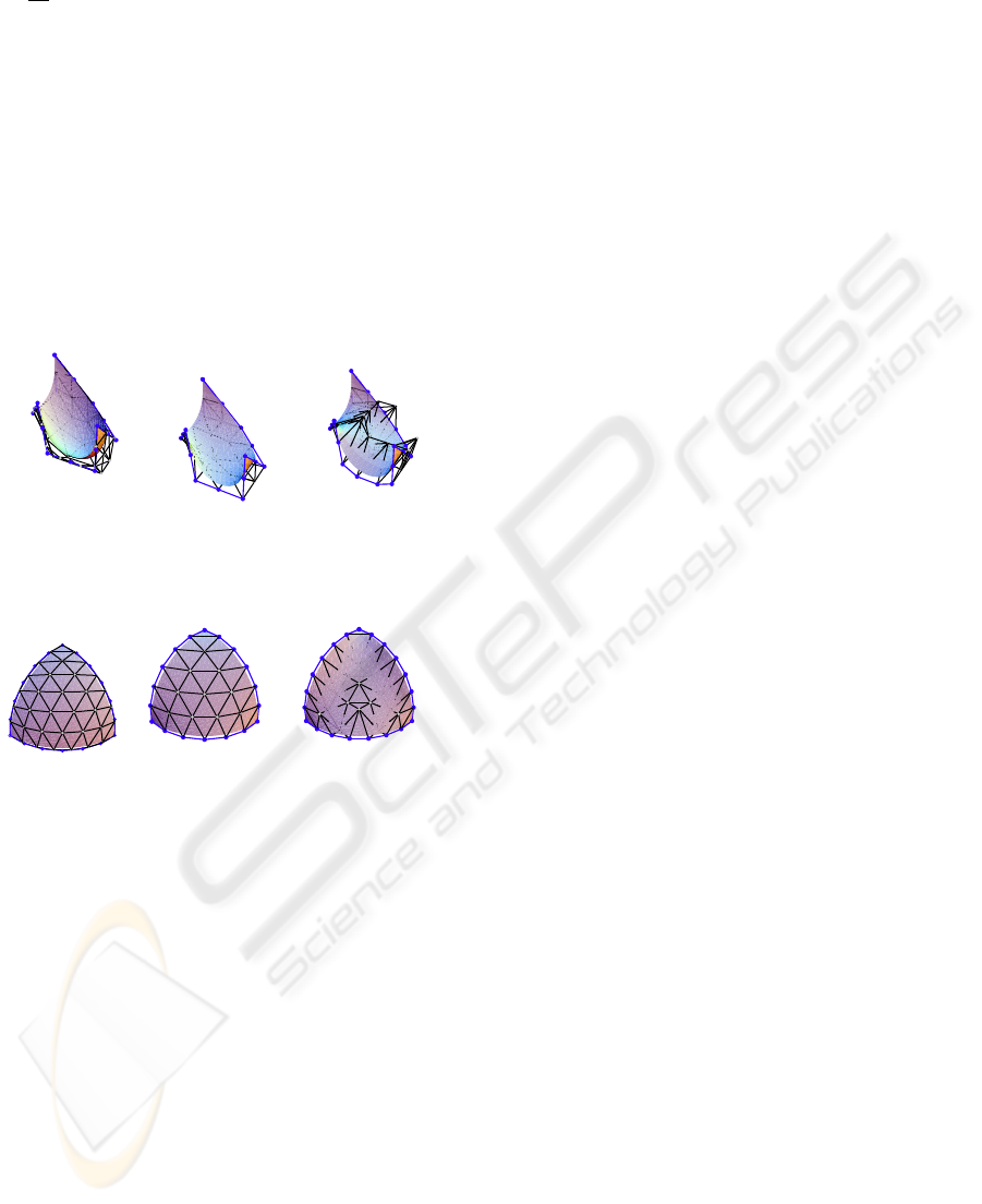
5 GRAPHICS EXAMPLES
Now, let us show some examples of the triangular
B
´
ezier surfaces we can obtain, given a boundary, by
means of the three different methods we have pre-
sented in this work: Coons interpolation, minimiza-
tion of the functional F and with the use of the mask
defined in Equation (11).
Figure 3: Three B
´
ezier surfaces with the same border. On
the left the triangular Coons patch. The one in the middle
is a B
´
ezier extremal of the functional F . The figure on the
right is obtained by means of the mask in Equation (11).
Figure 4: Three more examples of B
´
ezier triangles, the tri-
angular Coons patch, the B
´
ezier extremal of F in the middle
and the B
´
ezier surface built with the mask (11).
From the previous figures it can be seen that the
control nets obtained by means of the mask, in Equa-
tion (11), derived from the functional F are quite ir-
regular in comparison with the nets obtained as ex-
tremals of the functional.
6 CONCLUSIONS
Here we have conducted a study of one of the
most important solutions to the problem of finding
a surface interpolating boundary curves: triangular
Coons patches in comparison with rectangular Coons
patches. We have described three different surface
generation methods that start out from prescribed
boundary curves.
We have characterized the control net of a tri-
angular B
´
ezier extremal of the functional F . From
this characterization we have developed two meth-
ods to generate triangular patches given the boundary
curves. The first method is to find the extremals of
the functional as a solution of a linear system of the
control points. The second method makes it possible
to build a B
´
ezier triangle by means of a mask deduced
from the characterization of cubical extremals.
On the other hand, we have defined the Triangu-
lar Discrete Coons patch and we have compared the
shapes of the surfaces obtained by these three surface
generation methods. We have observed that better re-
sults are obtained for the extremals of the functional
and for the triangular Coons patch, but the Coons
patch implies an increase of degree.
ACKNOWLEDGEMENTS
We would thank to J. Monterde for his careful reading
of the paper and his valuable comments and sugges-
tions which helped to improve and clarify it.
This work has been partially supported by DGI-
CYT grant MTM2009-14500-C02-02.
REFERENCES
Arnal, A., Lluch, A., and Monterde, J. (2003). Triangu-
lar b
´
ezier surfaces of minimal area. In ICCSA (3),
volume 2669 of Lecture Notes in Computer Science,
pages 366–375. Springer.
Arnal, A., Lluch, A., and Monterde, J. (2008). Triangular
b
´
ezier approximations to constant mean curvature sur-
faces. In ICCS (2), volume 5102 of Lecture Notes in
Computer Science, pages 96–105. Springer.
Coons, S. A. (1967). Surfaces for computer aided design of
space forms. Technical Report MAC-TR-41, MIT.
Farin, G. and Hansford, D. (1999). Discrete Coons patches.
Comput. Aided Geom. Design, 16(7):691–700. Dedi-
cated to Paul de Faget de Casteljau.
Monterde, J. (2003). The plateau-b
´
ezier problem. In IMA
Conference on the Mathematics of Surfaces, volume
2768 of Lecture Notes in Computer Science, pages
262–273. Springer.
Monterde, J. (2004). B
´
ezier surfaces of minimal area: the
Dirichlet approach. Comput. Aided Geom. Design,
21(2):117–136.
Monterde, J. and Ugail, H. (2004). On harmonic and bihar-
monic B
´
ezier surfaces. Comput. Aided Geom. Design,
21(7):697–715.
Monterde, J. and Ugail, H. (2006). A general 4th-order pde
method to generate b
´
ezier surfaces from the boundary.
Computer Aided Geometric Design, 23(2):208–225.
Nielson, G. M., Thomas, D., and Wixom, J. (1978). Bound-
ary data interpolation on triangular domains. Tech-
nical Report GMR-2834, General Motors Research
Laboratories.
COONS TRIANGULAR BÉZIER SURFACES
153