
ADAPTIVE SEGMENTATION OF CELLS AND PARTICLES IN
FLUORESCENT MICROSCOPE IMAGES
Birgit M¨oller, Oliver Greß
Institute of Computer Science, Martin-Luther-University Halle-Wittenberg
Von-Seckendorff-Platz 1, 06099 Halle/Saale, Germany
Nadine St¨ohr, Stefan H¨uttelmaier
ZAMED, Martin Luther University Halle-Wittenberg
Stefan Posch
Institute of Computer Science, Martin Luther University Halle-Wittenberg
Keywords:
Active contours, Snakes, Wavelets, Segmentation, Fluorescent microscope images.
Abstract:
Microscope imaging is an indispensable tool in modern systems biology. In combination with fully automatic
image analysis it allows for valuable insights into biological processes on the sub-cellular level and fosters
understanding of biological systems. In this paper we present two new techniques for automatic segmentation
of cell areas and included sub-cellular particles. A new cascaded and intensity-adaptive segmentation scheme
based on coupled active contours is used to segment cell areas. Structures on the sub-cellular level, i.e. stress
granules and processing bodies, are detected applying a scale-adaptive wavelet-based detection technique.
Combining these results allows for complementary analysis of biological processes. It yields new insights into
interactions between different particles and distributions of particles among different cells. Our experimental
evaluations based on ground-truth data prove the high-quality of our segmentation results regarding these aims
and open perspectives towards deeper insights into biological systems on the sub-cellular level.
1 INTRODUCTION
Advances in fluorescence microscopy imaging allow
to study processes at a cellular level and supply a
valuable source of information for modern systems
biology. One of the questions which can be ap-
proached by this technique is the analysis of differ-
ent sub-cellular particles in eucaryotic cells which are
amongst others thought to be places of distinct func-
tions. Two kinds of such sub-cellular particles are
processing bodies (PBs) and stress granules (SGs),
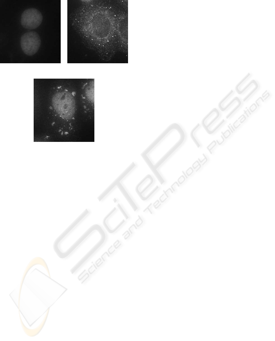
see Figure 1 for example image clips.
PBs are suggested to be places of mRNA degrada-
tion in eucaryotic cells as enzymes of the degradation
machinery are enriched in these foci (Eulalio et al.,
2007). However, if this function indeed can be re-
ferred to the particles remains elusive. The second
class of foci are SGs emerging during cellular stress
conditions (Yamasaki and Anderson, 2008). SGs are
assumed to be essential for mRNA storage during
stress (Yamasaki and Anderson, 2008), although this
presumption needs to be validated as well. To study
if or to what extent visible SGs and PBs can be con-
nected to a function within the cell it is essential to
monitor their occurrence. It is particularly of inter-
est in which cells of a given cell population the par-
ticles appear and if and how they interact with each
other. Also their distribution inside the different cells
yields valuable information for biological investiga-
tions. To answer these questions the need arises to not
only automatically detect PBs and SGs in microscope
images, but also to segment complete cell areas.
In biomedical experiments sub-cellular particles
of interest are fluorescently labeled in different chro-
matographic bands yielding multi-channel images
which are subsequently analyzed by automatic image
97
Möller B., Greß O., Stöhr N., Hüttelmaier S. and Posch S. (2010).
ADAPTIVE SEGMENTATION OF CELLS AND PARTICLES IN FLUORESCENT MICROSCOPE IMAGES.
In Proceedings of the International Conference on Computer Vision Theory and Applications, pages 97-106
DOI: 10.5220/0002849100970106
Copyright
c
SciTePress
(a) (b)
(c)
Figure 1: Fluorescently labeled nuclei and sub-cellular par-
ticles: (a) two cell nuclei, (b) a cell with labeled PBs, and
(c) one with labeled SGs.
analysis techniques. Unfortunately explicit labeling
of the complete cell area is typically not possible and
enforces to extract it from one of the available chan-
nels originally intended for detection of other parti-
cles. In our experimental data each image contains
three channels. In the nucleus channel of the images
nuclei manifest themselves by more or less homoge-
neously textured bright blobs. PBs are small bright
spots with a quite small variance in size while SGs
are usually significantly larger than PBs and show a
large variance in size (cf. Fig. 1).
Due to the significant variation in appearance of
the different sub-cellular particles there is no inte-
grated segmentation approach that allows to detect all
kinds of particles and the cells themselves. Accord-
ingly, we apply two different techniques for detect-
ing PBs and SGs on the one hand, and the cell ar-
eas on the other. PBs and SGs detection relies on a
scale-adaptive wavelet-based detection approach able
to cope with the variance in size of these particles
(Greß et al., 2010). Cell area segmentation is con-
ducted in the fluorescence channel for PBs in each
image. To solve the task we adopt coupled active con-
tour models.
One main contribution of this paper is the scale-
adaptive extension of a wavelet-based particle de-
tection algorithm. As the second main contribution
we present an extension of active contour models
towards a new cascaded segmentation scheme that
yields larger flexibility in segmenting objects with
specific intensity distributions. In detail, since the tar-
get area of a cell does not show significant disconti-
nuities along its border and also cannot be modeled
by one homogeneous intensity distribution, custom-
ary active contour energy models are not appropri-
ate to solve the given task. Our new cascaded ap-
proach overcomes these problems and allows to cope
with objects of non-homogeneous intensity distribu-
tions and weak discontinuities along their borders by
incremental adaptation to the objects’ intensity char-
acteristics.
The remainder of this paper is organized as fol-
lows. After reviewing related work in the next sec-
tion, we introduce our scale-adaptive wavelet-based
approach to particle detection in Section 3. In Sec-
tion 4 the new cascaded technique for intensity-
adaptivecell segmentation is presented. Subsequently
experimental evaluations based on ground-truth data
are discussed (Section 5), and we conclude with some
final remarks in Section 6.
2 RELATED WORK
Segmentation of cells and detection of particles in flu-
orescently labeled microscopy images are instances
of general problems in image analysis. Due to the spe-
cial characteristics of these images, adaptations are
required and have been proposed.
In (Dzyubachyk et al., 2007) and (Dzyubachyk
et al., 2008) a level-set based approach for segmen-
tation and tracking of cells is proposed. For initial
segmentation in the first time frame, the fitting term of
the classical Chan-Vese model (Chan and Vese, 2001)
is replaced with a Gaussian likelihood for the inten-
sity values with unknown variance. Lumped cells are
separated using the watershed transform and subse-
quent region merging. For tracking a multi phase
level-set technique is used employing a coupling term
of multiple level-set functions as proposed in (Dufour
et al., 2005). Approaching cells are separated via the
Radon-Transform in addition to the coupling term.
Several approaches exist for the detection of spot-
like particles, e.g. still using global and local thresh-
olding techniques like Otsu’s global method or the lo-
cal Niblack operator (Xavier et al., 2001; Bolte and
Cordelieres, 2006). Further techniques include sam-
pling from an image intensity density estimated via
h-dome transform and subsequent clustering of sam-
ples (Smal et al., 2008). The method in (Olivo-Marin,
2002; Genovesio et al., 2006) is based on wavelet de-
composition, but best-suited to detect particles with
VISAPP 2010 - International Conference on Computer Vision Theory and Applications
98
(a) (b) (c) (d)
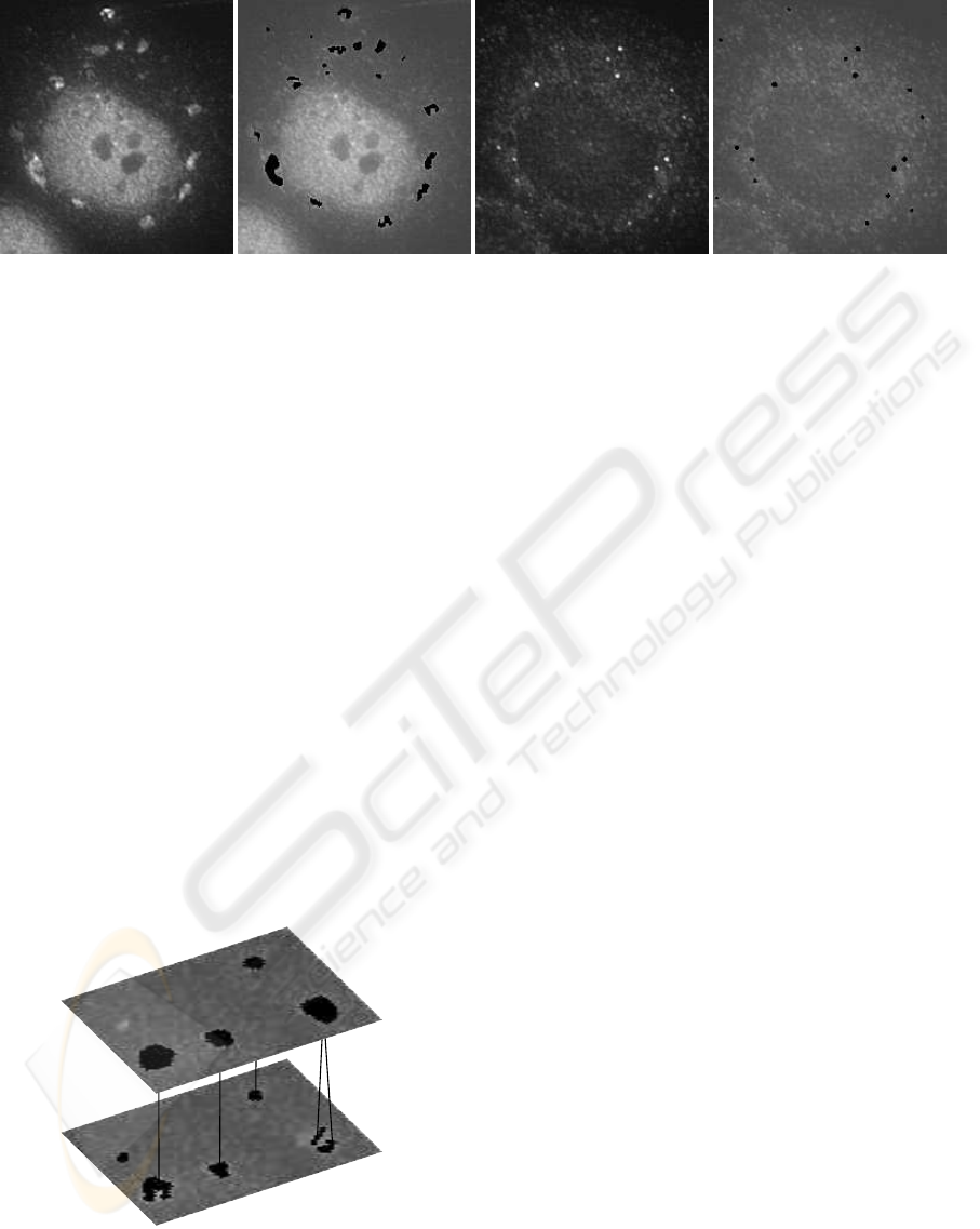
Figure 2: Examples of fluorescently labeled particles. (a) SG channel. (b) Detected SGs (black) using the scale-adaptive
wavelet algorithm. (c) PB channel. (d) Detected PBs (black) using the same algorithm. Image intensity values in (b) and (d)
are scaled for better visualization of detected particles.
limited variation in size.
An integrated algorithm for cell area segmentation
and sub-cellular particle detection was proposed by
(Dufour et al., 2008). They combine wavelet-based
particle detection adopting the approach of (Olivo-
Marin, 2002) with active contour-based cell area seg-
mentation. Unfortunately their snake energy is not
transferable to our domain as the cells in our sce-
nario show quite inhomogeneous and grainy intensity
distributions which do not allow for easy modeling
within a snake energy functional.
3 DETECTION OF PARTICLES
To detect particles in microscopy images we recently
proposed (Greß et al., 2010) to extend the method of
(Olivo-Marin, 2002; Genovesio et al., 2006), because
more flexibility with regard to size of particles to be
detected is required by the nature of stress granules.
Figure 3: Hypotheses trees for a clip of two correlation
images.
Detection as suggested in (Olivo-Marin, 2002)
uses the a trous wavelet transform on basis of third
order B-spline wavelets yielding wavelet coefficients
W
s
(x,y) = I
s
(x,y) − I
s−1
(x,y), s ∈ {1,...S}, (1)
where s denotes the scale and I
1
(x,y),...,I
S
(x,y) are
recursively smoothed versions of the original input
image I
0
(x,y).
Denoised wavelet coefficients
˜
W
s
(x,y) are ob-
tained applying the amplitude-scale-invariant Bayes
estimator (Figueiredo and Nowak, 2001). Wavelet
coefficients of adjacent scales are highly correlated
across scales due to the nature of the wavelet trans-
form applied, which motivates the combination of ad-
jacent scales s ∈ [a,b] to correlation images
c
[a,b]
(x,y) =
b
∏
s=a
˜
W
s
(x,y). (2)
Regions with large values in the correlation image are
assumed to correspond to particles, thus, finding con-
nected components after global thresholding yields
the detection result.
Particles of a certain size are best represented in a
particular interval of scales, therefore one interval is
appropriate if all particles in the image share similar
size characteristics. However, if a single scale interval
does not properly match the characteristics of the par-
ticles to be detected, irrelevant scales are included or
important ones are excluded, causing incorrect sizes
or shapes in detection, or leading to complete loss of
particles.
The use of multiple correlation images of – usu-
ally overlapping – scale intervals [a
n
,b
n
] allows the
detection of a particle in the scale interval which best
suits its characteristics. However, in many cases the
particle is also found in adjacent intervals with incor-
rect size or shape. This causes spatially overlapping
and thus competing particle hypotheses from different
scale intervals, from which we need to select the cor-
rect one. Overlapping and thus competing hypothe-
ses are organized in a tree with leaves corresponding
ADAPTIVE SEGMENTATION OF CELLS AND PARTICLES IN FLUORESCENT MICROSCOPE IMAGES
99

to the finest scale interval where hypotheses are avail-
able. Coarser scale hypotheses appear closer to the
root, as illustrated in Fig. 3.
The concept of meaningful events (Desolneux
et al., 2003) is employed to delete nodes of inferior
hypotheses from the tree. This meaningfulness can be
understood as the significance of an event produced
by a background process or under a null hypothe-
sis respectively, and has strong relation to statistical
hypothesis testing. The background process H
0
em-
ployed in our model assumes that no particle exists at
the present location and correlation image values are
caused by noise. Correlation values are supposed to
be pairwise independent, which allows us to represent
the probability P(F
i
| H
0
) that particle F
i
is produced
by the background process H
0
as
P(F
i
|H
0
) =
∏
(x,y)∈F
i
P
C
[a
n
,b
n
]
(x,y) = c
[a
n
,b
n
]
(x,y)|H
0
,
where C
[a
n
,b
n
]
(x,y) are random variables modeling the
correlation value for interval [a
n
,b
n
] observed at pixel
position (x,y). We denote with p(F
i
) the p-value of
F
i
, which is the probability to observe correlation val-
ues at least as extreme as the values of F
i
produced by
H
0
:
p(F
i
) =
∏
(x,y)∈F
i
P
C
[a
n
,b
n
]
(x,y) ≥ c
[a
n
,b
n
]
(x,y) | H
0
.
The tree of competing hypotheses is reduced com-
paring p-values. To account for the difference in size
of the support of hypotheses, the p-value of a node is
normalized by the size of its support. Starting from
the leaves, a parent’s normalized p-value is compared
to the product of the normalized p-values of its chil-
dren. Hypotheses with smaller p-values are kept as
they are assumed to be more unlikely caused by noise.
The described method is able to select detection
candidates from the correct scale interval. Examplary
detection results for SGs and PBs are shown in Fig. 2
where SGs are hypothesized in intervals [2,3] and
[3,4] and selected from the appropriate interval ac-
cording to their size.
4 CELL SEGMENTATION
4.1 Snake Basics
Active contours can either be modeled implicitly
adopting level-set approaches or explicitly in terms
of parametric contour models, i.e. snakes. While the
numerical tractability of level-set approaches is often
superior compared to snake optimization techniques,
topology preservation is usually easier to guarantee
by snake approaches as topological stability is inher-
ent in the model theory underlying snakes. In our sce-
nario the number of objects to segment is known in
advance, hence the topology of the desired segmenta-
tion result is known. For this reason we prefer explicit
active contour models for this application.
In explicit approaches the contour of an object is
defined as a function c : R → R
2
which maps a param-
eter value s ∈ [0,1] defined along a given contour c
to points (x,y) in 2-D space. For object segmentation
an energy functional over the contour function c(s) is
defined. The contour is evolved towards a local min-
imum of the energy, which gives the final segmenta-
tion result.
In general the energy functional of an explicit ac-
tive contour consists of two types of energy terms.
On the one hand we have an internal energy term
E
int
(c(s)) solely depending on the contour itself,
e.g. its length and curvature,
E
int
(c(s)) =
1
2
Z
1
0
α· k c
′
(s) k
2
+β· k c
′′
(s) k
2
ds, (3)
where α and β are weighting constants. On the other
hand we have an external energy term which is usu-
ally derived from the input image to be segmented,
E
ext
(c(s)) =
Z
1
0
f
ext
(c(s))ds. (4)
During segmentation the snake is iteratively moved to
minimize the composed snake energy
E(c(s)) = E
int
(c(s)) + E
ext
(c(s)). (5)
The optimization procedure relies on implicit gradient
descent techniques, introducing a time t to model the
contour evolution process, and given Euler-Lagrange
formulations (Kass et al., 1988) of the snake energy
functional:
c
t
(s) = c
t−1
(s) −
1
γ
·
dE(c
t
(s))
dc
t
(s)
. (6)
γ denotes the step-size for the gradient descent step in
each iteration.
4.2 Region Homogeneity Criterium
In contrast to several related papers on cell segmenta-
tion for fluorescent microscope images our target ob-
jects, i.e. the cell areas, are not characterized by sig-
nificant gray-scale discontinuities along their bound-
aries. Rather they show specific region intensity pro-
files (cf. Fig. 4 (a)). Accordingly, widely used exter-
nal snakes energies like gradient-based terms do not
provide helpful information for our application. We
therefor replace E
ext
as defined in Eq. 4 by a snake en-
ergy term proposed in (Chan and Vese, 2001) which
VISAPP 2010 - International Conference on Computer Vision Theory and Applications
100
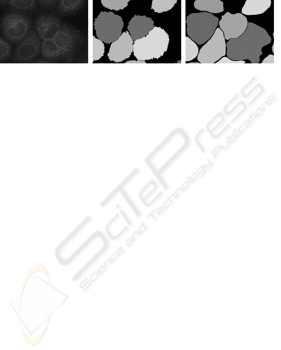
(a) (b) (c)
Figure 4: Example image clip showing (a) dark nuclei surrounded by cell area and fluorescently labeled PBs, (b) the mask
corresponding to the automatic segmentation result, and (c) the manually labeled ground-truth mask for comparison.
considers not only image intensity information along
the snake itself but also intensity data of the complete
image domain Ω. In particular, the intensities for the
interior and exterior regions of the snake, R
in
(c(s))
and R
out
(c(s)) respectively, are modeled as constant
and are denoted by c
in
and c
out
. Deviations from these
constant intensities are penalized as follows:
E
r
(c(s)) = λ
in
·
Z
R
in
(c(s))
(I(x, y) − c
in
)
2
dΩ
+λ
out
·
Z
R
out
(c(s))
(I(x, y) − c
out
)
2
dΩ, (7)
where I(x,y) is the input image intensity at pixel po-
sition (x,y) and λ
in
and λ
out
are weighting constants.
During optimization this term pushes the snake to a
location where its interior pixel value distribution is
well described by c
in
, and the remaining exterior pixel
value distribution by c
out
. It is noted that this model
of constant intensities and quadratic error terms is
approximately equivalent to a Gaussian model with
means c
in
and c
out
and standard deviations λ
in
and
λ
out
, see e.g. (Dzyubachyk et al., 2007).
4.3 Snake Coupling
The typical use case of snake-based segmentation as-
sumes a single snake to be optimized within a given
image at a single point in time. For our application,
however, we aim at segmenting a set of multiple cells.
In particular, information about the contour of one
cell directly effects the contour of neighboring cells.
Most importantly it has to be ensured that snakes do
not overlap which would correspond to overlapping
cells that do not occur in reality. Consequently, proper
segmentation of the complete image is only possible
by performing an integrated optimization of all cell
contours in parallel. We adopt the approach of (Zim-
mer and Olivo-Marin, 2005) and introduce a common
energy functional E
c
for N snakes including internal
snake energies (Eq. 3), region homogeneity criteria
(cf. Eq. 7) and an energy term that allows to penalize
overlapping snake regions:
E
c
(c
1
(s),...,c
N
(s)) =
N
∑
i=1
E
int
(c
i
(s))
+λ
in
·
N
∑
i=1
Z
R
in
(c
i
(s))
I(x, y) − c
i
in
2
dΩ
+λ
out
·
Z
Ω\(
S
N
i=1
R
in
(c
i
(s)))
(I(x, y) − c
out
)
2
dΩ
+ρ ·
N
∑
i=1
N
∑
j=i+1
Z
R
in
(c
i
(s))∩R
in
(c
j
(s))
1dΩ . (8)
The last summand considers for each pair of snakes
(c
i
(s),c
j
(s)) the area of interior overlap R
in
(c
i
(s)) ∩
R
in
(c
j
(s)) and weights it with a constant ρ.
For optimization the Euler-Lagrange functional
with regard to each single snake c
i
(s) is derived yield-
ing N evolution equations in total. These are individ-
ually optimized following the implicit approach pro-
posed in Eq. 6.
4.4 Cascaded Active Contours
Analyzing the general appearance of cells in our ap-
plication it becomes obvious that their region inten-
sity distribution cannot very well be modeled by a
Gaussian intensity distribution underlying E
r
in Eq. 7.
Rather several rings of approximately Gaussian inten-
sity value distributions can be identified enclosing the
central nucleus region of a cell (cf. Fig. 4 (a)). The
average intensities of these rings monotonically de-
crease from the nucleus region towards the outer sec-
tions of the cell.
Due to this intensity distribution of cells the above
model is not very well suited to segmented a complete
cell. One option is to adapt the intensity model for
cell regions according to intensity profiles observed.
However, this is quite difficult as not only more so-
phisticated intensity distributions like Gaussian mix-
tures need to be integrated, but also the characteristic
ADAPTIVE SEGMENTATION OF CELLS AND PARTICLES IN FLUORESCENT MICROSCOPE IMAGES
101
spatial variationsof the intensity values require proper
consideration.
As an alternative we apply a cascaded segmenta-
tion approach. For initialization we detect nucleus re-
gions and use their contours as initial snakes for the
cells. The segmentation process consists of three sub-
sequent levels of snake optimization. Each level aims
at extending the current segmentation result towards
the next outward intensity ring of the cell.
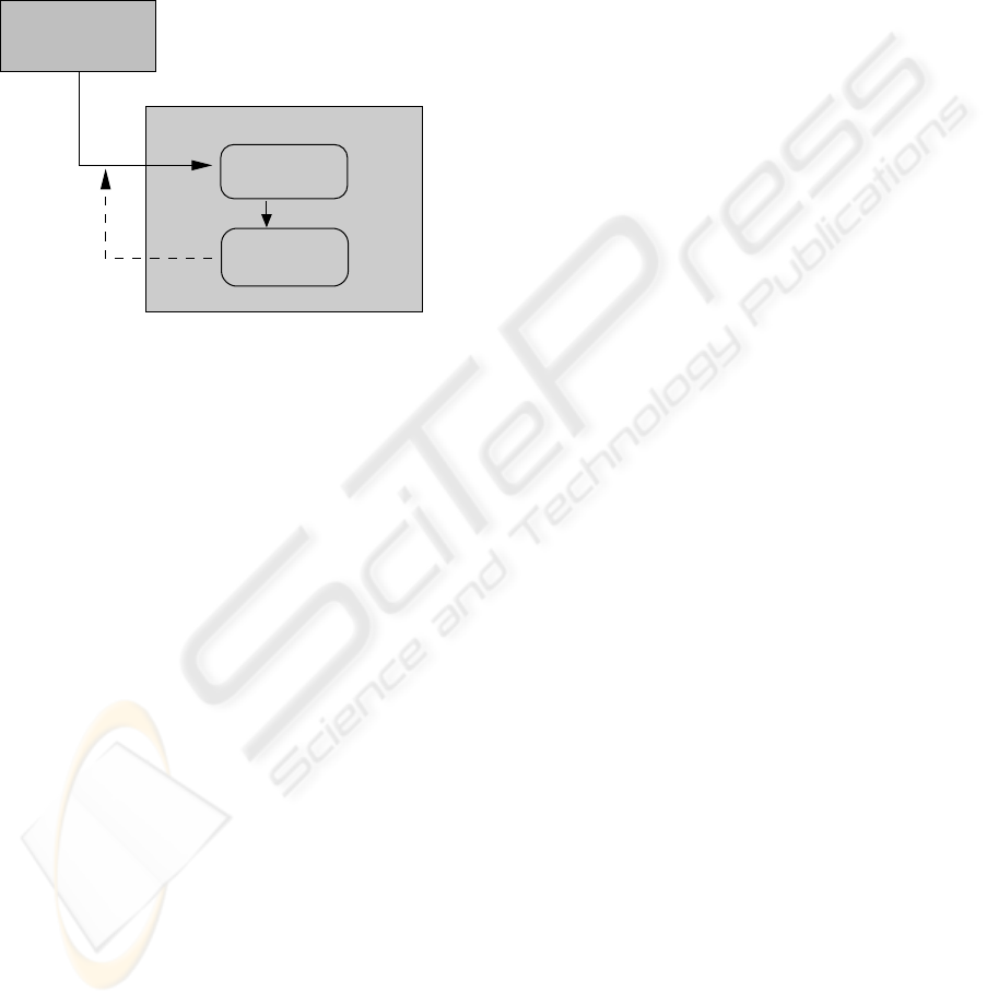
Initialization:
Otsu thresholding
of nuclei regions
Segmentation Level l:
Iterative snake
optimization
snake interiors
N snake
contours
contours
initial
Dilation of initial
for level l+1
average intensities c_in
Figure 5: Overview of the cascaded segmentation approach.
Fig. 5 shows a diagram of the cascaded segmenta-
tion algorithm with its three levels. The initial nucleus
segmentation is accomplished using a global Otsu’s
thresholding followed by morphological closing. For
each connected component a cell is hypothesized and
its contour yields an initial snake.
At the beginning of each segmentation level l the
interior of each initial snake contour for this level
is dilated by 10 pixels. This dilation is constraint
to avoid overlap between neighboring snakes. From
each expanded image region of approximately 10
pixel width the average intensity is extracted for snake
c
n
(s) and used as initial constant c
l,n
in
for the subse-
quent optimization level.
As this initial average intensity tends to be smaller
than c
l−1,n
in
extracted during the previoussegmentation
level, the snake is driven to evolve towards the outside
for integrating the new darker regions into the cell.
Each snake finally converges to a position where its
overall energy is minimized according to Eq. 8. This
result is subsequently used as contour initialization
in the subsequent segmentation level. In conclusion,
each snake incrementally includes darker regions into
its area, and finally stops at the border to the back-
ground of the outmost lying intensity ring.
5 RESULTS
In the following we discuss experimental results of
our cascaded segmentation approach. In particular,
we will show the high quality of the cell segmentation
by comparing our results to manually labeled ground-
truth data. For PBs and SGs the assignment to indi-
vidual cells is assessed given automatic and ground-
truth cell segmentation.
5.1 Image Data
The algorithm was evaluated on 5 sample images
resulting from a common experimental setup. The
cells stem from the human hepatoma cell line (HUH7
cells). Each image consists of three channels, contain-
ing fluorescently labeled nuclei, SGs and, PBs respec-
tively. SGs are labeled by immunostaining of TIAR
(a protein localized in SGs), while PBs are labeled by
immunostaining of DCP1a (decapping enzyme local-
ized in PBs). The nuclei are labeled by DAPI.
In total, all images include 86 cells manually la-
beled for ground-truth. Initial snakes for the snake
segmentation are derived from detected cell nuclei as
explained above. It may happen during nuclei de-
tection that nuclei located very close to each other
are fused into a single nucleus region. In such cases
snakes are missing, i.e. not all ground-truth cells can
properly be segmented with the given set of initial
snakes. To nevertheless enable a fair evaluation of the
snake segmentation approach and due to the fact that
the automatic nucleus detection algorithm is not part
of this contribution, the labeling of ground-truth cells
was adapted accordingly for such cells. In detail, if
two or three nuclei merged during automatic segmen-
tation also the cells involved were merged in manual
ground-truth labeling. After adaptation 77 ground-
truth cells remain for evaluation.
5.2 Segmentation Results
The cascaded segmentation algorithm was applied
with three levels, each with its own parameter settings
(Tab. 1). Note that for all images and each of the three
levels the same set of parameters was applied.
When optimizing snakes in practice one important
issue to ensure accurate and comparable localization
properties at each point position along the contour is
to keep the distance between subsequent points of the
snake, i.e. the length of the snake segments, more or
less uniform. In our approach the snake is parameter-
ized with the desired segment length l
seg
, and every
second iteration the segments are checked and in case
VISAPP 2010 - International Conference on Computer Vision Theory and Applications
102
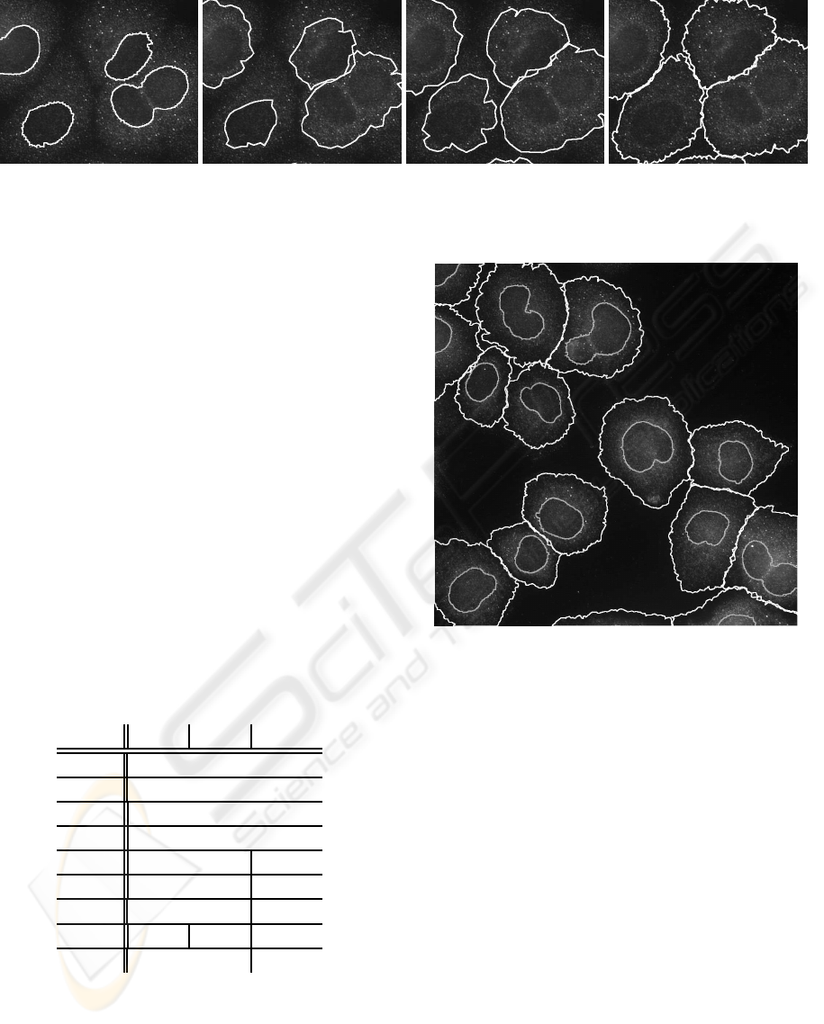
(a) (b) (c) (d)
Figure 6: Cropped image section showing the evolution of the snake starting with the initial snakes extracted from the nucleus
regions (a) and the results of subsequent optimization levels 1 to 3 (b-d).
of large deviations from the optimum segment length
points are added or deleted accordingly.
The snake is supposed to stop in a locally optimal
energy state, i.e. a position of minimal snake energy.
In our setup we use a combination of two stopping
criteria for checking if the snake converged. On the
one hand we analyze the relative change in the area of
snake interior between two iterations and stop opti-
mization if it falls below a certain threshold value ∆A.
In addition, a maximum number of admissible itera-
tions I
max
is defined mainly to prevent the snake from
oscillating between two steady states with difference
in area size just below the threshold ∆A.
In general, during the first two levels the overall
shape of the cells is extracted. In level 3 accurate lo-
cal segmentation and local improvements with regard
to low intensity regions get higher priority. Accord-
ingly the weight of the curvature term is increased,
the length of the contour segments is decreased and
the stopping criteria are adapted.
Table 1: Parameters used during snake segmentation.
Level: 1st 2nd 3rd
λ
in
0.1
λ
out
25
ρ 10000
α 1.25
β 0.75 1.25
γ 0.0001 0.0002
l
seg
15 5
∆A 0.015 0.005 0.001
I
max
100 200
Prototypical segmentation results of our approach
are shown in Figs. 4, 6 (d), and 7. Comparing the two
image clips in Fig. 4 (b) and (c) showing overall seg-
mentation result and ground-truth, it is obvious that
the overall segmentation result is satisfactory. Par-
ticularly the segmentation of cell boundaries in con-
glomerating sets of cells is of high quality. In outer
Figure 7: Cell segmentation result on complete image, final
contours are shown in white, initial nuclei contours in gray.
sections of the cells sometimes fractions of the cell
area are still missing. However, as the figures below
indicate the missing sections only marginally degrade
the quality of the results. This is due to the fact that
for our application the main focus is the correct as-
signment of PBs and SGs to cells, and the distribution
of their numbers and localization with respect to the
cells and their nuclei.
The main idea of our 3-level approach is to itera-
tively improve segmentation results. During level one
large parts of the cell are still missing, while in lat-
ter levels almost the complete cell area is included in
the segmentation result. This is exemplary shown in
Figure 6 for a clip of one image which also demon-
strates the incremental improvement of cell segmen-
tation, which cannot be achieved in one single snake
segmentation run. Fig. 7 shows final cell contours
as extracted by our new approach for a complete im-
age of the test set emphasizing again the high perfor-
mance of the algorithm in adequately separating con-
glomerating cells.
ADAPTIVE SEGMENTATION OF CELLS AND PARTICLES IN FLUORESCENT MICROSCOPE IMAGES
103
Cell segmentation can be regarded a classification
task on the pixel level. For optimal results each pixel
of a labeled ground-truth cell should be segmented by
the algorithm and correctly classified into the correct
cell class. These pixels correctly classified as cell pix-
els are the true positives (TP), while pixels incorrectly
classified as cell pixels are false positives (FP). Pixels
incorrectly classified as background or belonging to
other cells are false negatives (FN). Based on this in-
terpretation for each ground-truth cell, precision and
recall can be calculated. The recall TP/(TP + FN)
is defined as the ratio of ground-truth pixels that were
actually correctly detected by the segmentation algo-
rithm, while the precision TP/(TP + FP) gives the
ratio of detected cell pixels that are actually lying in-
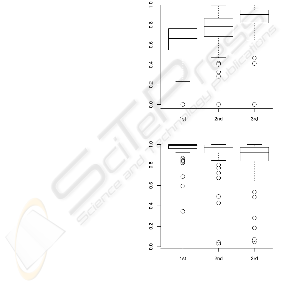
side ground-truth cells. In Figures 8 and 9 box-plots
for the recall and precision achieved are presented.
For each of the three segmentation levels the values
are shown, in each case averaged over all 77 cells.
Considering the recall its median steadily in-
creases from 0.66 after the first segmentation level to
0.79 and finally 0.91 after the last level. This is due to
the fact that beginning with the initial nucleus region
in each level the algorithm segments larger fractions
of the cells.
For the precision the tendency is just conversely.
Since the initial cell regions are derived from the
nuclei segmented, the contours from the first level
predominately lie completely within the surrounding
cells, i.e. very few false negatives appear in the seg-
mentation. With evolving snake contours the cell area
grows, and consequently the chance to include pix-
els into the snake region that actually belong to the
background or other cells increases. The precision de-
creases from an initial median of 0.99 to a final value
of 0.92. Note that for more than 75% of the cells the
value still exceeds 0.84.
In both plots outliers with recall and precision val-
ues close to zero can be observed. On the one hand
these result from very small cells that are enclosed
into the area of significantly larger cells in their neigh-
borhoodduring segmentation resulting in a significant
amount of false positives and small precision, respec-
tively. One the other hand the outlier cell with very
low recall values relates to a ground-truth cell located
near the image boundary where only small fractions
of the cell nucleus are visible. Consequently the ini-
tial snake contains only very few polygon points and
rapidly collapses rather than to segment the cell. Alto-
gether precision and recall indicate that the segmenta-
tion misses some fractions of several cells, but barely
includes additional non-cell pixels.
From the biological point of view besides the ac-
tual automatic detection of PBs and SGs one very
valuable information is the distribution of the parti-
cles with regard to the cells. In detail, different bio-
logical implications result if the particles are equally
spread over all cells of a sample or quite inhomoge-
neously distributed in the cell population. Therefore
we assess the assignment of the PBs and SGs to the
different cells compared to ground-truth cell segmen-
tation. In Figures 10 and 11 the corresponding scatter
plots are shown.
Figure 8: Average recall values for all 77 cells.
Figure 9: Average precision values for all 77 cells.
On the abscissa of each plot the number of par-
ticles, either PBs or SGs, in a ground-truth cell is
shown, on the ordinate the automatically detected
number of PBs or SGs in the corresponding cell seg-
mented via snakes is outlined. In case of optimal par-
ticle assignment from correctly segmented cell areas
VISAPP 2010 - International Conference on Computer Vision Theory and Applications
104
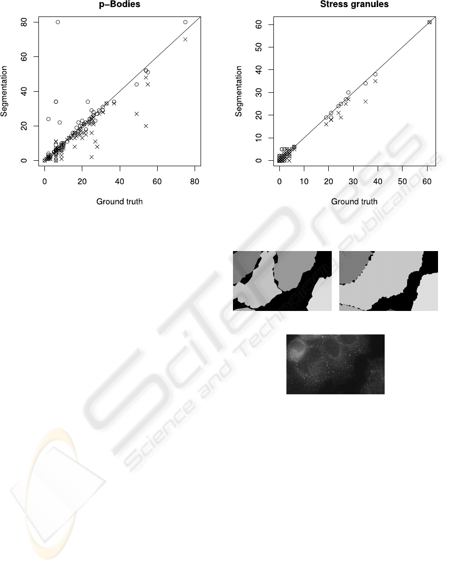
Figure 10: Number of cooccurring PBs in ground-truth and
segmented cells after the first segmentation level (cross) and
in the final result (circle).
the plots should show a perfect bisecting line. In both
plots the results after the first iteration are shown as
crosses, while the final results are marked by circles.
Note that in the setup of the biological experiment
the number of SGs in the images is in general signif-
icantly smaller than the number of PBs. Nevertheless
in both plots it is clearly visible that the cooccurence
increases. Regarding SGs the Spearman rank correla-
tion coefficient slightly increases from 0.852 to 0.888.
Also for PBs the majority of data points moves
towards the bisecting line. The correlation value de-
creases from initially 0.891 to 0.853 and finally 0.832.
The main reason for this are two collapse events dur-
ing segmentation leading to wrong cell correspon-
dences. In both cases at the beginning a set of three
ground-truth cells is corresponding to exactly three
snake contours. In the course of the segmentation,
however, one of the snakes collapses and the cell is in-
cluded in the area of a neighboring snake (cf. Fig. 12).
Consequently a single segmented cell corresponds to
two ground-truth cells, whereas only one of them is
the correct one while the second ground-truthcell gets
assigned many false positive detection results. In the
plot in Fig. 10 the outlier point in the top left corner
of the plot is caused by one of these events.
6 CONCLUSIONS
We proposed two techniques for automatic analysis
of fluorescence microscopy images: one algorithm to
segment the areas of cells, and a second one for the
Figure 11: Number of cooccurring SGs in ground-truth and
segmented cells after the first segmentation level (cross) and
in the final result (circle).
(a) (b)
(c)
Figure 12: Example for segmentation failure. While in level
2 (a) three snake regions model the ground-truth cells, in
level 3 (b) one snake disappears allowing one of the remain-
ing two to wrongly occupy its region as well. Note that the
cells are hard to separate even manually (c).
detection of sub-cellular particles, namely PBs and
SGs. For particle detection we extend an approach
based on correlated wavelet coefficients from the a
trous wavelet transform. To accommodate particles of
varying size we introduce a set of scale intervals and
resolve ambiguities in the resulting particle hypothe-
ses by adapting the concept of meaningful events.
Secondly, for the segmentationof cell areas composed
of nested rings of decreasing intensities we expand
a coupled active contour model into a cascaded seg-
mentation technique. The core idea of this technique
is to incrementally incorporate the intensity rings into
the segmentation result, starting with the nucleus of
ADAPTIVE SEGMENTATION OF CELLS AND PARTICLES IN FLUORESCENT MICROSCOPE IMAGES
105

each cell as initialization. Our algorithms are evalu-
ated on a set of 5 images with cells of a human hep-
atoma cell line, each composed of three channels la-
beling nuclei, SGs and PBs, respectively. The results
clearly show the benefits of the cascaded approach as
the overall segmentation quality is high. This is true
as well for precision and recall of cell areas as for the
assignment of particles to their corresponding cells.
Future work will include improvements of nucleus
segmentation to avoid or correct fusion of neighbor-
ing nuclei. Furthermore, data-depended adaption of
the number of levels used in the cascaded approach
with an appropriate stopping criterium will be scruti-
nized.
REFERENCES
Bolte, S. and Cordelieres, F. P. (2006). A guided tour
into subcellular colocalization analysis in light mi-
croscopy. Journal of Microscopy, 224(3):213–232.
Chan, T. and Vese, L. (2001). Active contours with-
out edges. IEEE Transactions on image processing,
10(2):266–277.
Desolneux, A., Moisan, L., and Morel, J.-M. (2003). A
grouping principle and four applications. IEEE Trans.
PAMI, 25(4):508–513.
Dufour, A., Meas-Yedid, V., Grassart, A., and Olivo-Marin,
J. (2008). Automated quantification of cell endocy-
tosis using active contours and wavelets. In Pattern
Recognition, 2008. ICPR 2008. 19th International
Conference on Pattern Recognition.
Dufour, A., Shinin, V., Tajbakhsh, S., Guillen-Aghion, N.,
Olivo-Marin, J., and Zimmer, C. (2005). Segment-
ing and tracking fluorescent cells in dynamic 3-D mi-
croscopy with coupled active surfaces. IEEE Transac-
tions on Image Processing, 14(9):1396–1410.
Dzyubachyk, O., Niessen, W., and Meijering, E. (2007).
A variational model for level-set based cell tracking
in time-lapse fluorescence microscopy images. In
IEEE International Symposium on Biomedical Imag-
ing. IEEE, Piscataway.
Dzyubachyk, O., Niessen, W., and Meijering, E. (2008).
Advanced level-set based multiple-cell segmentation
and tracking in time-lapse fluorescence microscopy
images. In IEEE International Symposium on Biomed-
ical Imaging. IEEE, Piscataway.
Eulalio, A., Behm-Ansmant, I., and Izaurralde, E. (2007). P
bodies: at the crossroads of post-transcriptional path-
ways. Nature Reviews Molecular Cell Biology, 8:9–
22.
Figueiredo, M. A. T. and Nowak, R. D. (2001). Wavelet-
based image estimation: an empirical bayes approach
using jeffrey’s noninformative prior. IEEE Trans. IP,
10(9):1322–1331.
Genovesio, A., Liedl, T., Emiliani, V., Parak, W., Coppey-
Moisan, M., and Olivo-Marin, J. (2006). Multiple
Particle Tracking in 3-D+ Microscopy: Method and
Application to the Tracking of Endocytosed Quantum
Dots. IEEE Transactions on Image Processing, 15(5).
Greß, O., M¨oller, B., St¨ohr, N., H¨uttelmaier, S., and Posch,
S. (2010). Scale-adaptive wavelet-based particle de-
tection in microscopy images. In Proceedings of the
Workshop Bildverarbeitung f¨ur die Medizin (BVM).
Springer. accepted for publication.
Kass, M., Witkin, A. P., and Terzopoulos, D. (1988).
Snakes: Active contour models. International Jour-
nal of Computer Vision, 1(4):321–331.
Olivo-Marin, J. (2002). Extraction of spots in biological im-
ages using multiscale products. Pattern Recognition,
35(9):1989–1996.
Smal, I., Niessen, W., and Meijering, E. (2008). A new
detection scheme for multiple object tracking in fluo-
rescence microscopy by joint probabilistic data asso-
ciation filtering. In 5th IEEE International Symposium
on Biomedical Imaging: From Nano to Macro, 2008.
ISBI 2008, pages 264–267.
Xavier, J., Schnell, A., Wuertz, S., Palmer, R., White, D.,
and Almeida, J. (2001). Objective threshold selection
procedure (OTS) for segmentation of scanning laser
confocal microscope images. Journal of microbiolog-
ical methods, 47(2):169.
Yamasaki, S. and Anderson, P. (2008). Reprogramming
mRNA translation during stress. Curr. Opin. Cell
Biol., 20:222–226.
Zimmer, C. and Olivo-Marin, J. (2005). Coupled parametric
active contours. IEEEtransactions on pattern analysis
and machine intelligence, 27(11):1838–1842.
VISAPP 2010 - International Conference on Computer Vision Theory and Applications
106
