
DIAGNOSIS OF ACTIVE SYSTEMS BY LAZY TECHNIQUES
Gianfranco Lamperti and Marina Zanella
University of Brescia, Dipartimento di Ingegneria dell’Informazione, Via Branze 38, 25123 Brescia, Italy
Keywords:
Diagnosis, Discrete-event systems, Active systems, Communicating automata, Uncertainty, Lazyness.
Abstract:
In society, laziness is generally considered as a negative feature, if not a capital fault. Not so in computer
science, where lazy techniques are widespread, either to improve efficiency or to allow for computation of
unbounded objects, such as infinite lists in modern functional languages. We bring the idea of lazy computation
to the context of model-based diagnosis of active systems. Up to a decade ago, all approaches to diagnosis of
discrete-event systems required the generation of the global system model, a technique that is impractical when
the system is large and distributed. To overcome this limitation, a lazy approach was then devised in the context
of diagnosis of active systems, which works with no need for the global system model. However, a similar
drawback arose a few years later, when uncertain temporal observations were proposed. In order to reconstruct
the system behavior based on an uncertain observation, an index space is generated as the determinization of a
nondeterministic automaton derived from the graph of the uncertain observation, the prefix space. The point is
that the prefix space and the index space suffer from the same computational difficulties as the system model.
To confine the explosion of memory space when dealing with diagnosis of active systems with uncertain
observations, a laziness-based, circular-pruning technique is presented. Experimental results offer evidence
for the considerable effectiveness of the approach, both in space and time reduction.
1 INTRODUCTION
Active systems (Lamperti and Zanella, 2003) are a
class of asynchronous discrete-event systems that can
be used to model, at a high abstraction level, real
physical systems in order to carry out diagnosis and
monitoring. In the last decade such tasks have been
investigated and a number of working algorithms have
been proposed (Baroni et al., 1999; Lamperti and
Zanella, 2004; Lamperti and Zanella, 2006). Before
the notion of active system were defined, synchronous
discrete-event systems had already been considered in
the literature as a promising modeling abstraction for
monitoring and diagnosis purposes (Sampath et al.,
1995; Sampath et al., 1996). What was actually more
innovative since the very initial introduction of active
systems (Baroni et al., 1998) was not, as is seemingly
obvious, the different class of modeled systems (asyn-
chronous vs. synchronous), but the ability to come to
a diagnosis without previously generating the global
behavioral model of the system, an ability which,
although dealt with for asynchronous discrete-event
systems, applies also to synchronous ones.
This ability may be considered as an instance of
a lazy computation, as opposed to a busy compu-
tation. In computer science laziness is a positive
feature, aimed at saving computational resources in
both space and time, which is adopted in several
contexts, such as Boolean expression evaluation and
functional languages, including Haskell (Thompson,
1999). Trivially, laziness obeys a general principle
which states that a processing step shall be performed
only if and when necessary. In the context of di-
agnosis of discrete-event systems, the global behav-
ioral model of the system, which encompasses all
the possible evolutions of the system, compliant with
whichever observation, is not strictly necessary in or-
der to reconstruct the dynamic evolutions based on
a given specific observation (as is the case in or-
der to solve a single diagnosis/monitoring problem).
Therefore, in a lazy perspective, the global behavioral
model is not built and only the evolutions compli-
ant with the given observation are reconstructed. If
the same diagnostic problem occurs several times, the
same on-line computation is performed in each ses-
sion. In a busy perspective, instead, the global behav-
ioral model is built off-line once and for all and then
it is exploited for all diagnostic sessions, bringing a
considerable gain in on-line computational complex-
ity. The reason for a lazy computation is to be pre-
171
Lamperti G. and Zanella M. (2010).
DIAGNOSIS OF ACTIVE SYSTEMS BY LAZY TECHNIQUES.
In Proceedings of the 12th International Conference on Enterprise Information Systems - Artificial Intelligence and Decision Support Systems, pages
171-180
DOI: 10.5220/0002855101710180
Copyright
c
SciTePress

Figure 1: Fragment of power transmission network.
Therefore, i n a lazy perspective, the global behavioral
model is not built and only the evolutions compli-
ant with the given observation are reconstructed. If
the same diagnostic prob lem occurs several times, th e
same on-line computation is performed in each ses-
sion. In a busy perspective, instead, the global behav-
ioral model is built off-line once and for all and then
it is exploited for all diagnostic sessions, bringing a
considerable gain in on-line computational complex-
ity. The reason for a lazy computation is to be pre-
ferred i s that the size of t he global behavio ral model i s
explosive for real-scale systems, thus a busy app roach
is practically infeasible. That is why all state-of-the-
art approaches to diagnosis of discrete-event systems
(Pencol´e and Cordier, 2005) do not rely on the gener-
ation of the global behavioral sy stem model.
Some years aft er the introduction of active sys-
tems, the concept of a temporal uncertain observa-
tion was defined (Lamperti and Zanella, 2002), and
diagnosis problems featuring such a kind of observa-
tions were taken into account. An uncertain tempo-
ral observation, b ei ng under-constrained, represents
several sequences of observable events. For diagno-
sis purposes, all the evolutions of the active system,
consistent with all such sequences, have to be recon-
structed on-li ne. Such a reconstruction is driven by
a deterministic acyclic automaton, called the index
space, which is obtained as the determinization of an
acyclic automaton, called th e prefix space, which, in
turn, is drawn from a directed acyclic graph, which i s
the mor e natural fr ont-end representation of an uncer-
tain observation.
The approaches proposed so far to diagnose an ac-
tive system given a temporal uncertain observation
suppose that the whole index space is built, neces-
sarily on-l ine since the observation may vary over
sessions. However, the size of the prefix space and
the index space is huge even for small observation
graphs, therefore such approaches are practically in-
feasible. Moreover, such spaces may include paths
that are physically impossible, that is, sequences of
observable events that cannot be generated by the
considered active system. The approaches proposed
so far can then be considered as busy ones from the
point of view of observation handling, while this pa-
per proposes a lazy approach for di agnosis of active
systems with uncertain temporal observations, that is,
an approach that builds only the useful portions of the
prefix space and the index-space (and avoids build-
ing physically i mpossible states). Envisaging such an
approach is not straightforward since one can realize
that a path of the index space is physically impossi-
ble, and , therefore, it has to be pru ned, only based
on the reconstruction of the evolutions of the system.
Thus a circularity arises: on the one hand, the index
space drives the evolution reconstruction and, on the
other, the performed reconstruction serves as a basis
for discardin g states in the index space and in the pre-
fix space as well. How to cope with this circularity is
the purpose of this paper.
2 APPLICATION DOMAIN
Supervision of power networks is the application
domain for which diagnosis of act ive systems was
first conceived. A power network is composed o f
transmission lines. Each transmission line is pro-
tected by two breakers that are commanded by a pro-
tection. The protection is designed to detect the oc-
currence of a short circuit on the line based on the
continuous measurement of its impedance: when the
impedance goes beyond a given threshold, the two
breakers are commanded to open, thereby causing
the extinction of the short circuit. In a simplified
view, the network is represented by a series of lines,
each one associated with a protection, as displayed
in Fig. 1, where lines l
1
l
4
are protected by pro-
tections p
1
p
4
, respectively. For inst ance, p
2
con-
trols l
2
by operating breakers b
21
and b
22
. In normal
(correct) behavior, bo th breakers are expected to open
when tripped by the protection. However, the protec-
tion system may exhibit an abnormal (faulty) behav-
ior, for example, one breaker or both may not o pen
when required. In such a case, each faulty breaker in-
forms the protection about its own misbehavior. Then,
the protection sends a request of recovery actions to
the neighboring protections, which will operate their
own breakers appropriately. For example, if p
2
oper-
ates b
21
and b
22
and th e latter is f aulty, then p
2
will
send a signal to p
3
, which is su pposed to command
Figure 1: Fragment of power transmission network.
ferred is that the size of the global behavioral model is
explosive for real-scale systems, thus a busy approach
is practically infeasible. That is why all state-of-the-
art approaches to diagnosis of discrete-event systems
(Pencol
´
e and Cordier, 2005) do not rely on the gener-
ation of the global behavioral system model.
Some years after the introduction of active sys-
tems, the concept of a temporal uncertain observa-
tion was defined (Lamperti and Zanella, 2002), and
diagnosis problems featuring such a kind of observa-
tions were taken into account. An uncertain tempo-
ral observation, being under-constrained, represents
several sequences of observable events. For diagno-
sis purposes, all the evolutions of the active system,
consistent with all such sequences, have to be recon-
structed on-line. Such a reconstruction is driven by
a deterministic acyclic automaton, called the index
space, which is obtained as the determinization of an
acyclic automaton, called the prefix space, which, in
turn, is drawn from a directed acyclic graph, which is
the more natural front-end representation of an uncer-
tain observation.
The approaches proposed so far to diagnose an ac-
tive system given a temporal uncertain observation
suppose that the whole index space is built, neces-
sarily on-line since the observation may vary over
sessions. However, the size of the prefix space and
the index space is huge even for small observation
graphs, therefore such approaches are practically in-
feasible. Moreover, such spaces may include paths
that are physically impossible, that is, sequences of
observable events that cannot be generated by the
considered active system. The approaches proposed
so far can then be considered as busy ones from the
point of view of observation handling, while this pa-
per proposes a lazy approach for diagnosis of active
systems with uncertain temporal observations, that is,
an approach that builds only the useful portions of the
prefix space and the index-space (and avoids build-
ing physically impossible states). Envisaging such an
approach is not straightforward since one can realize
that a path of the index space is physically impossi-
ble, and, therefore, it has to be pruned, only based
on the reconstruction of the evolutions of the system.
Thus a circularity arises: on the one hand, the index
space drives the evolution reconstruction and, on the
other, the performed reconstruction serves as a basis
for discarding states in the index space and in the pre-
fix space as well. How to cope with this circularity is
the purpose of this paper.
2 APPLICATION DOMAIN
Supervision of power networks is the application do-
main for which diagnosis of active systems was first
conceived. A power network is composed of trans-
mission lines. Each transmission line is protected by
two breakers that are commanded by a protection.
The protection is designed to detect the occurrence
of a short circuit on the line based on the continuous
measurement of its impedance: when the impedance
goes beyond a given threshold, the two breakers are
commanded to open, thereby causing the extinction
of the short circuit. In a simplified view, the network
is represented by a series of lines, each one associ-
ated with a protection, as displayed in Fig. 1, where
lines l
1
···l
4
are protected by protections p
1
··· p
4
, re-
spectively. For instance, p
2
controls l
2
by operating
breakers b
21
and b
22
. In normal (correct) behavior,
both breakers are expected to open when tripped by
the protection. However, the protection system may
exhibit an abnormal (faulty) behavior, for example,
one breaker or both may not open when required. In
such a case, each faulty breaker informs the protec-
tion about its own misbehavior. Then, the protection
sends a request of recovery actions to the neighboring
protections, which will operate their own breakers ap-
propriately. For example, if p
2
operates b
21
and b
22
and the latter is faulty, then p
2
will send a signal to
p
3
, which is supposed to command b
32
to open. A re-
covery action may be faulty on its turn. For example,
b
32
may not open when tripped by p
2
, thereby caus-
ing a further propagation of the recovery to protection
p
4
. The protection system is designed to propagate
the recovery request until the tripped breaker opens
correctly. When the protection system is reacting, a
subset of the occurring events are visible to the oper-
ator in a control room who is in charge of monitoring
the behavior of the network and, possibly, to issue ex-
plicit commands so as to minimize the extent of the
isolated sub-network. Generally speaking, the local-
ization of the short circuit and the identification of the
faulty breakers may be impractical in real contexts,
ICEIS 2010 - 12th International Conference on Enterprise Information Systems
172

especially when the extent of the isolation spans sev-
eral lines and the operator is required to take recovery
actions within stringent time constraints. On the one
hand, there is the problem of observability: the ob-
servable events generated during the reaction of the
protection system are generally uncertain in nature.
On the other, it is impractical for the operator to rea-
son on whatever observation so as to make consistent
hypotheses on the behavior of the system and, eventu-
ally, to establish the shorted line and the faulty break-
ers.
3 DIAGNOSIS TASK
An active system is a network of components that are
connected to one another through links. Each compo-
nent is modeled by a communicating automaton that
reacts to events either coming from the external world
or from neighboring components. Events exchanged
between components are queued into links before be-
ing consumed. The way a system reacts to an event
coming from the external world is constrained by the
communicating automata of the involved components
and the way such components are connected to one
another. The whole set of evolutions of a system Σ,
starting at the initial state σ
0
, is confined to a finite au-
tomaton, the behavior space of Σ, Bsp(Σ,σ
0
). How-
ever, a strong assumption for diagnosis of active sys-
tems is the unavailability of the behavior space since,
in real, large-scale applications, the generation of the
behavior space is impractical. As such, Bsp(Σ,σ
0
) is
intended for formal reasons only. A (possibly empty)
path within Bsp(Σ,σ
0
) rooted in σ
0
is a history of Σ.
When the system reacts, it performs a sequence of
transitions within the behavior space, called the ac-
tual history of the system. Some of these transitions
are observable as visible labels. Also, each transition
can be either normal or faulty. If faulty, the transition
is associated with a faulty label. Given a history h,
the (possibly empty) set of faulty labels encompassed
by h is the diagnosis entailed by h. Likewise, the se-
quence of visible labels encompassed by h is the trace
of h.
Example 1. Shown in Fig. 2 is an abstraction of the
behavior space Bsp(Σ,σ
0
). We assume that each arc
corresponds to a component transition, which moves
the system from one state to another. In the fig-
ure, only the visible labels of observable transitions,
namely a, b, and c, are displayed. A possible history
is [σ
0
,σ
2
,σ
4
,σ
2
,σ
4
,σ
6
,σ
8
], with trace [a,c,b].
Ideally, the reaction of a system should be ob-
served as the trace of the actual history. However,
b
32
to open. A recovery action may be faulty on its
turn. For example, b
32
may not open wh en tripped
by p
2
, thereby causing a further propagation of the
recovery to protection p
4
. The protection system is
designed t o propagate the recovery request until the
tripped breaker opens correctly. When the protection
system is reacting, a subset of the o ccurring events
are visible to the operator in a control room who is in
charge of monitoring the behavior of the network and,
possibly, to issue explicit commands so as to mini-
mize the extent of t he isolated sub-network. Gener-
ally speaking, the localization of the short circuit and
the identification of the faulty breakers may be im-
practical in real contexts, especially when th e extent
of the i solation spans several lines and the operator is
required to take recovery actions within stringent time
constraints. On th e one hand, there is the p roblem of
observability: the observable events generated during
the reaction of the protection syst em are generally un-
certain in nature. On the other, it is impractical for
the operator to reason on whatever observat ion so as
to make consistent hypotheses on the behavior of the
system and, event ually, to establish the shorted line
and the faulty breakers.
3 DIAGNOSIS TASK
An active system is a network of component s that
are connected to on e another throu gh links. Each
component is modeled by a communicating automa-
ton that reacts to events either coming from the exter-
nal world or from neighboring components. Events
exchanged between components are queued into links
before being consumed. The way a system reacts
to an event coming from the external world is con-
strained by the communicating automata of the in-
volved components and the way such components are
connected to one another. The whole set of evolu-
tions of a system ˙, starting at the initial state
0
,
is confined to a finite automaton, the behavior space
of ˙, Bsp.˙;
0
/. However, a strong assumption for
diagnosis of active systems is the unavailabil ity o f
the behavior space since, in r eal, large-scale applica-
tions, the generation of the behavior space is imprac-
tical. As such, Bsp.˙;
0
/ is intended for formal rea-
sons only. A (possibly empty ) p at h within Bsp.˙;
0
/
rooted in
0
is a history of ˙. When the system r e-
acts, it performs a sequence of transitions within the
behavior space, called the actual history of the sys-
tem. Some of these transitions are observable as visi-
ble labels. Al so, each transition can be either normal
or faulty. If faulty, the transition is associated with a
faulty label. Given a hist ory h, the (possibly empty)
Figure 2: Behavior space Bsp.˙;
0
/.
set of faulty labels encompassed by h is the diagnosis
entailed by h. Likewise, the sequence of visible labels
encompassed by h is the trace of h.
Example 1. Shown in Fig. 2 is an abstraction of the
behavior space Bsp.˙ ;
0
/. We assume that each arc
corresponds to a component transition, which moves
the system from one state to another. In the fig-
ure, only the visible labels of o bservable transitions,
namely a, b, and c, are displayed. A possible history
is Œ
0
;
2
;
4
;
2
;
4
;
6
;
8
, with trace Œa; c; b.
Ideally, the reaction of a system should be ob-
served as the trace of the actual history. However,
what is actually observed is a temporal o bservation
O. This is a directed acyclic graph, where nodes are
marked by sets of candidate visible labels, while arcs
denote partial temporal ordering among nodes. For
each node, only one label is the actual label (the one
in the actual history), with the others being the spuri-
ous l abels. The set of labels in a node ! o f O is de-
noted as k!k. Since temporal ordering is only partial,
several candidate traces are possib le for O, with each
candidate being determined by cho osing a label f or
each n ode while respecting the ordering constraints
imposed by arcs. The set of candidate traces is writ-
ten kOk.
Example 2. Depicted in Fig. 3 is a temporal obser-
vation O involving nodes !
1
; : : :; !
4
. Node !
2
is
marked by labels b and , where the latter is the null
label, which is in fact invisible. Thus, as far as !
2
is concerned, either b or nothing has been generated
by the system. Since !
3
and !
4
are connected by an
arc, c necessarily precedes this occurrence of b in any
trace. Note that trace Œa; c; b belo ngs to kOk.
A diagnostic problem }.˙/ requi res determining
the set of candidat e diagnoses implied by the histories
of ˙ whose traces are in kOk. Intuitively, the (pos-
sibly infinite) set of hi stories in Bsp.˙;
0
/ is filtered
based on the constraints imposed by each trace rele-
vant to O. Since among such traces is the (unknown)
Figure 3: Temporal observation O for system ˙ .
Figure 2: Behavior space Bsp(Σ,σ
0
).
what is actually observed is a temporal observation
O. This is a directed acyclic graph, where nodes are
marked by sets of candidate visible labels, while arcs
denote partial temporal ordering among nodes. For
each node, only one label is the actual label (the one
in the actual history), with the others being the spuri-
ous labels. The set of labels in a node ω of O is de-
noted as kωk. Since temporal ordering is only partial,
several candidate traces are possible for O, with each
candidate being determined by choosing a label for
each node while respecting the ordering constraints
imposed by arcs. The set of candidate traces is writ-
ten kOk.
Example 2. Depicted in Fig. 3 is a temporal obser-
vation O involving nodes ω
1
,...,ω
4
. Node ω
2
is
marked by labels b and ε, where the latter is the null
label, which is in fact invisible. Thus, as far as ω
2
is concerned, either b or nothing has been generated
by the system. Since ω
3
and ω
4
are connected by an
arc, c necessarily precedes this occurrence of b in any
trace. Note that trace [a,c,b] belongs to kOk.
b
32
to open. A recovery acti on may be faulty on its
turn. For example, b
32
may not open when tripped
by p
2
, thereby causing a further propagation of t he
recovery to protection p
4
. The protection system is
designed to propagate the recovery request until the
tri pped breaker opens correctly. When the pr otection
system is reacting, a subset of the occurring events
are visible to the operator in a control room who is in
charge of monitoring the behavio r of the network and,
possibly, to issue explicit commands so as to mini-
mize the extent of t he isolated sub-network. Gener-
ally speaking, the localization of the short circui t and
the identificat ion of the faulty breakers may be im-
practical in real contexts, especially when t he extent
of the isolation spans several lines and the operator is
required to take recovery actions within stringent time
constraints. On the one hand, there is the problem of
observability: the observabl e events generated durin g
the reaction of the protection system are generally un-
certain in natur e. On the other, it is impractical for
the operator t o reason on whatever observation so as
to make consistent hypotheses on the behavior of the
system and, eventually, to establ ish the shorted line
and the faulty breakers.
3 DIAGNOSIS TA SK
An active system is a network of components that
are connected to one another through links. Each
component is modeled by a communicating automa-
ton that reacts to events either coming from the exter-
nal world or from neighboring components. Events
exchanged betw een components are queued into links
before b ei ng con sumed. The way a sy stem reacts
to an event coming from the external world is con-
strained by the communicating automata of the in-
volved components and the way such components are
connected to one another. The whole set of evolu-
tions of a system ˙, starting at the initial state
0
,
is confined to a fini te automaton, the behavior space
of ˙, Bsp.˙;
0
/. However, a strong assumption for
diagnosis of active systems is the unavailability of
the behavior space since, in real, large-scale applica-
tions, the generat ion of the behavior space is imprac-
tical. As such, Bsp.˙;
0
/ is intended for formal rea-
sons only. A (possi bly empty) path within Bsp.˙;
0
/
rooted in
0
is a hist ory of ˙. When the system re-
acts, it performs a sequence of transitions within the
behavior space, called the actual history of the sys-
tem. Some of these transitions are observable as visi -
ble labels. Also, each transiti on can be either normal
or faulty. If faulty, the transition is associated with a
faulty label. Given a history h, the (possibly empty)
Figure 2: Behavior space Bsp.˙;
0
/.
set of faulty labels encompassed by h is the diagnosis
entailed by h. Likewise, the sequence of visible labels
encompassed by h is the trace of h.
Example 1. Shown in Fig. 2 is an abstractio n of the
behavior space Bsp.˙;
0
/. We assume that each arc
corresponds to a component transition, w hich moves
the system from one state to another. In the fig-
ure, on ly the visible labels of observable transitions,
namely a, b, and c, are displayed. A possible history
is Œ
0
;
2
;
4
;
2
;
4
;
6
;
8
, with trace Œa; c; b.
Ideally, the reaction of a system should be ob-
served as the trace of the actual history. However,
what is actually observed is a temporal ob servation
O. This is a directed acyclic graph, where nodes are
marked by sets o f candidate visible labels, while arcs
denote partial temporal ordering among nodes. For
each n ode, only one label is th e actual label (the one
in the actual history), with the oth ers being th e spuri-
ous labels. The set of labels in a node ! of O is de-
noted as k!k. Since temporal ordering is only partial,
several candidate traces are possible for O, wi th each
candidate being determined by choosing a label for
each no de while respecting the ordering constraints
imposed b y arcs. The set of candidate traces is writ-
ten kOk.
Example 2. Depicted in Fig. 3 is a temporal obser-
vat ion O involving nodes !
1
; : : :; !
4
. Node !
2
is
marked by labels b and , where the latter is the null
label, which is in fact invisible. Thus, as far as !
2
is concerned, either b or nothing has been generated
by the system. Since !
3
and !
4
are connected by an
arc, c necessarily precedes this occurrence of b in any
trace. Note that trace Œa; c; b belongs to kOk.
A diagnostic problem }.˙/ requ ires determining
the set of candidate diagnoses i mplied by the histories
of ˙ whose traces are in kOk. Intuitively, the (po s-
sibly infini te) set of histories in Bsp.˙;
0
/ is filtered
based on the constraints imposed by each trace rele-
vant to O. Since among such traces is the (unknown)
Figure 3: Temporal observation O for system ˙ .
Figure 3: Temporal observation O for system Σ.
A diagnostic problem ℘(Σ) requires determining
the set of candidate diagnoses implied by the histories
of Σ whose traces are in kOk. Intuitively, the (possi-
bly infinite) set of histories in Bsp(Σ,σ
0
) is filtered
based on the constraints imposed by each trace rele-
vant to O. Since among such traces is the (unknown)
actual trace, among the candidate diagnoses will be
the diagnosis implied by the actual history, namely
the (unknown) actual diagnosis. To solve ℘(Σ), the
diagnostic engine performs three major steps:
1. Indexing. An index space Isp(O) is generated
from O. This is a deterministic automaton whose
regular language is kOk.
2. Reconstruction. Based on Isp(O), the set of histo-
ries whose trace is in kOk is determined in terms
of a behavior, written Bhv(℘(Σ)). This is an au-
tomaton such that each state is a pair (σ,ℑ), where
σ is a state in Bsp(Σ, σ
0
) and ℑ a state in Isp(O).
A transition (σ,ℑ)
T
−→ (σ
0
,ℑ
0
) in Bhv(℘(Σ)) is
DIAGNOSIS OF ACTIVE SYSTEMS BY LAZY TECHNIQUES
173
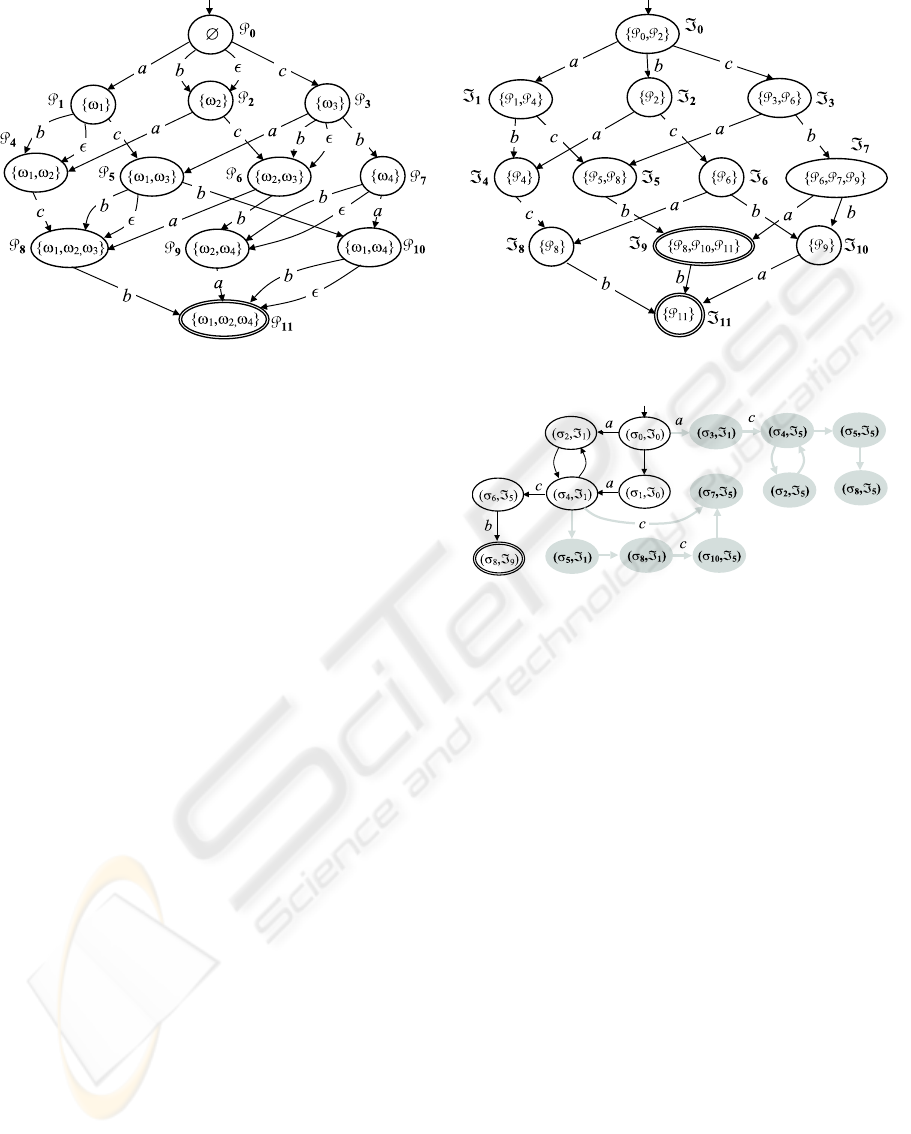
Figure 4: Prefix space Psp.O/ (left) and index space Isp.O/ (right).
actual trace, among the candidate diagnoses will be
the diagnosis implied by the actual histor y, namely
the (unknown) actual diagnosis. To solve }.˙/, the
diagnostic engine performs three major steps:
1. Indexing. An index space Isp.O/ is generated
from O. This is a deterministic automaton whose
regular language is kOk.
2. Reconstruction. Based on Isp.O/, the set of histo-
ries whose trace is in kOk is determined in terms
of a behavior, written Bhv.}.˙//. This is an au-
tomaton such that each state is a pair .; =/, where
is a state in Bsp.˙;
0
/ and = a state in Isp .O/.
A transiti on .; =/
T
! .
0
; =
0
/ in Bhv.}.˙// is
such that
T
!
0
is a transition in Bsp.˙;
0
/.
Besides, if T is visible with label `, then =
`
! =
0
is a transition in Isp.O/, otherwi se =
0
D =.
3. Decoration. Each state in Bhv.}.˙/ is decorated
by the set of diagnoses implied by all histories
ending at such a state.
Eventually, the solution of }.˙/ is determined by dis-
tilling the diagn oses, in the decorated behavi or, whose
state is associated with a final state of Isp.O/.
Example 3. Outlined on the ri ght-h and side of Fig. 4
is the index space of observation O (Fig. 3 ), n amely
Isp.O/. This is generated as the determinization of
a nondetermin istic automaton called the prefix space
of O, written Psp.O/, outlined on the left-hand side.
Each state P of Psp.O/ is a set of nodes of O, called
a prefix of O. A prefix P implicitly identifies P
,
where P
is the union of P and the set of ancesto rs
(in O) of all nodes in P . For instance, P
9
identifies
f!
2
; !
4
g [ f !
3
g. Psp.O/ is generated starting from
the empty set P
0
and, for each state P , select ing one
node ! 2 O not included in P
, whose ancestors are
included in P
. Then, for each label ` 2 k!k, a transi-
tion P
`
! P
0
is inserted, where P
0
is the prefix iden-
tifying the set P
[ f!g. Only one final state exists,
(in our example, P
11
), identifying all nodes of O.
Example 4. Shown in Fig. 5 is the reconstructed be-
havior (plain part of the graph) relevant to a diagnostic
problem }.˙/, wh ere the behavior space of ˙ is in
Fig. 2, the observation O in Fig. 3, and the index space
of O in Fig. 4. The gray part of the graph is generated
by the reconstruction al gorithm, but is eventuall y dis-
carded as spurious (since i t is not encompassed by any
path from initial state .
0
; =
0
/ to final state .
8
; =
9
/.
Notice that the regular language of Bhv.}.˙// is the
singleton fŒa; c; bg, despite the infinite number of his-
tories (owing to cycles).
The previous example shows that the language of
Bhv.}.˙// is a subset of the l anguage of Isp.O/. Pre-
cisely, the language of the reconstructed behavior is
the intersection of the lang uage of the index space and
the language of the b ehavior space.
Figure 5: Reconstruction o f behavior Bhv.}.˙ //.
Figure 4: Prefix space Psp(O) (left) and index space Isp(O) (right).
such that σ
T
−→ σ
0
is a transition in Bsp(Σ,σ
0
). Be-
sides, if T is visible with label `, then ℑ
`
−→ ℑ
0
is a
transition in Isp(O), otherwise ℑ
0
= ℑ.
3. Decoration. Each state in Bhv(℘(Σ) is decorated
by the set of diagnoses implied by all histories
ending at such a state.
Eventually, the solution of ℘(Σ) is determined by dis-
tilling the diagnoses, in the decorated behavior, whose
state is associated with a final state of Isp(O).
Example 3. Outlined on the right-hand side of Fig. 4
is the index space of observation O (Fig. 3), namely
Isp(O). This is generated as the determinization of
a nondeterministic automaton called the prefix space
of O, written Psp(O), outlined on the left-hand side.
Each state P of Psp(O) is a set of nodes of O, called a
prefix of O. A prefix P implicitly identifies P
∗
, where
P
∗
is the union of P and the set of ancestors (in O) of
all nodes in P . For instance, P
9
identifies {ω
2
,ω
4
} ∪
{ω
3
}. Psp(O) is generated starting from the empty
set P
0
and, for each state P , selecting one node ω ∈ O
not included in P
∗
, whose ancestors are included in
P
∗
. Then, for each label ` ∈ kωk, a transition P
`
−→ P
0
is inserted, where P
0
is the prefix identifying the set
P
∗
∪{ω}. Only one final state exists, (in our example,
P
11
), identifying all nodes of O.
Example 4. Shown in Fig. 5 is the reconstructed be-
havior (plain part of the graph) relevant to a diagnos-
tic problem ℘(Σ), where the behavior space of Σ is in
Fig. 2, the observation O in Fig. 3, and the index space
of O in Fig. 4. The gray part of the graph is generated
by the reconstruction algorithm, but is eventually dis-
carded as spurious (since it is not encompassed by any
path from initial state (σ
0
,ℑ
0
) to final state (σ
8
,ℑ
9
).
Notice that the regular language of Bhv(℘(Σ)) is the
Figure 4: Prefix space Psp.O/ (left) and index space Is p.O/ (right).
actual trace, among the candidate diagnoses will be
the diagnosis impl ied by the actual history, namely
the (unknown) actual diagnosis. To solve }.˙/, the
diagnostic engine performs three major steps:
1. Indexing. An index space Isp.O/ is generated
from O. This is a deterministic aut omaton whose
regular language is kOk.
2. Reconstruction. Based on Isp.O/, the set of histo-
ries whose trace is in kOk is determined in terms
of a behavior, written Bhv.}.˙//. This is an au-
tomaton such that each state is a pair .; =/, where
is a state in Bsp.˙;
0
/ and = a st at e in Isp.O/.
A transition .; =/
T
! .
0
; =
0
/ in Bhv.}.˙// is
such that
T
!
0
is a transition in Bsp.˙;
0
/.
Besides, if T is visible with label `, then =
`
! =
0
is a transition in Isp.O/, otherwise =
0
D =.
3. Decoration. Each state in Bhv.}.˙/ is decorated
by the set of diagnoses implied by all histories
ending at such a stat e.
Eventually, the solution o f }.˙/ is determined by dis-
tilling the diagno ses, in the decorated b ehavior, who se
state is associated with a final state of Isp.O/.
Example 3. Outlined on the right-hand side of Fig. 4
is the index space of observation O (Fig. 3), namely
Isp.O/. This is generated as the determinization of
a nondeterministic automaton called the prefix space
of O, written Psp.O/, outlined on the left-hand side.
Each state P of Psp.O/ is a set of nodes of O, called
a prefix of O. A prefix P implicitly identifies P
,
where P
is the union of P and the set of ancestors
(in O) of all nodes in P . For instance, P
9
identifies
f!
2
; !
4
g [ f!
3
g. Psp.O/ is generated starting from
the empty set P
0
and, for each state P , selecting one
node ! 2 O not included in P
, whose ancestors are
included in P
. Then, for each label ` 2 k!k, a transi -
tion P
`
! P
0
is inserted, where P
0
is the pr efix iden-
tif ying the set P
[ f!g. Only one final state exists,
(in our example, P
11
), identifying all nodes of O.
Example 4. Shown in Fig. 5 is the reconstructed be-
havior (plain p art of the graph) relevant to a diagnostic
problem }.˙/, where the behavior space of ˙ is in
Fig. 2, the observat ion O in Fi g. 3, and t he index space
of O in Fig. 4. The gray part of the graph is generated
by the reconstruction algorithm, but is eventually dis-
carded as spurious (since it is not encompassed by any
path from initial state .
0
; =
0
/ to fin al state .
8
; =
9
/.
Notice that the regular language of Bhv.}.˙// is the
singleton fŒa; c; bg, despite the infinite number of his-
tories (owing to cycles).
The previous example shows that the language of
Bhv.}.˙// is a subset of th e language of Isp.O/. Pre-
cisely, the language of the reconstru ct ed behavior is
the intersection of the language of the index space and
the language of the behavior sp ace.
Figure 5: Reconstruction of behavior Bhv.}. ˙ //.
Figure 5: Reconstruction of behavior Bhv(℘(Σ)).
singleton {[a, c, b]}, despite the infinite number of his-
tories (owing to cycles).
The previous example shows that the language of
Bhv(℘(Σ)) is a subset of the language of Isp(O). Pre-
cisely, the language of the reconstructed behavior is
the intersection of the language of the index space and
the language of the behavior space.
4 LAZY DIAGNOSTIC ENGINE
The systematic approach to problem solving intro-
duced above may become inappropriate owing to the
explosion of the prefix space and, consequently, of
the index space. This problem arose when experi-
menting with algorithms for subsumption-checking of
temporal observations (Lamperti and Zanella, 2008).
The cause for the huge number of nodes can be un-
derstood by analyzing how the index space is gener-
ated. Given an observation O, the prefix space of O is
built by considering all possible ways in which nodes
of O can be selected, based on the precedence con-
straints imposed by the arcs of O. At each choice,
we create new transitions in the prefix space, marked
by the labels within the selected node of O, and con-
ICEIS 2010 - 12th International Conference on Enterprise Information Systems
174

nect each of them to another state of Psp(O). Such
a state is marked by a set of nodes (a prefix) of O
that identifies the whole set of nodes already chosen in
O. Intuitively, the less temporally constrained O, the
larger the set of possible sequences of choices. The
exact number of states in Psp(O) equals the cardinal-
ity of the whole set of prefixes of O. In particular,
assuming n nodes in O, if O is linear (nodes totally
ordered) then the number of states in Psp(O) equals
n + 1. If O is totally disconnected (nodes temporally
unconstrained) then the number of states in Psp(O)
equals 2
n
. So, in the worst case, the number of states
of Psp(O) grows exponentially with the number of
nodes in O. In practice, even for disconnected ob-
servations of moderate size, say 40 nodes, the prefix
space contains 2
40
states, corresponding to more than
10
12
states! With such numbers, if the generation of
the prefix space is impractical, the transformation of it
into the equivalent deterministic automaton, the index
space, is simply out of question. So, what to do? Gen-
erally speaking, not all the candidate traces included
in Isp(O) are consistent with the behavior space of
the system, just as not all the histories included in the
behavior space are consistent with Isp(O). In fact,
in the reconstruction phase, we filter out the histo-
ries in Bsp(Σ,σ
0
) based on the constraints imposed by
Isp(O), thereby yielding Bhv(℘(Σ)). Now, the point
is, we might try to perform some sort of pruning of
the index space Isp(O) based on the constraints im-
posed by the behavior space Bsp(Σ,σ
0
). However,
this would work only assuming the availability of the
latter, which is not the case. A better idea is to filter
out the index space based on the reconstructed behav-
ior Bhv(℘(Σ)). This allows us to avoid the genera-
tion of Bsp(Σ,σ
0
). By contrast, the problem is now
that Bhv(℘(Σ)) is itself generated based on Isp(O),
giving rise to a circularity: we need Isp(O) to gen-
erate Bhv(℘(Σ)) and we need Bhv(℘(Σ)) to generate
Isp(O). Interestingly, we can cope with this circular-
ity by building the index space and the reconstructed
behavior adopting a lazy approach, where the con-
structions of the two automata are intertwined. So,
the reciprocal constraints can be checked at each step.
A second shortcoming of the systematic approach
to problem solving concerns the structure of the re-
constructed behavior.
• Let β = (σ, ℑ) be either the initial state or a state
reached by a visible transition in Bhv(℘(Σ)). Let
Silent(β) be the subgraph of Bhv(℘(Σ)) rooted in
β and reached by silent transitions only. Then, all
states in Silent(β) will share the same index ℑ.
• Let β
1
= (σ,ℑ
1
) and β
2
= (σ,ℑ
2
) be two states
in Bhv(℘(Σ)) sharing the same system state σ.
Then, the projections of Silent(β
1
) and Silent(β
2
)
Figure 4: Prefix space Psp.O/ (left) and index space Isp.O/ (right).
actual trace, among the candidate diagnoses will be
the diagnosis implied by the actual history, namely
the (unk nown) actual dia gnosis. To solve }.˙/, the
diagnostic engine performs three major steps:
1. Indexing. An index space Isp.O/ is generated
from O. This is a determin istic automaton whose
regular language is kOk.
2. Reconst ruction. Based on Isp .O/, the set of histo-
ries whose trace is in kOk is d etermined in terms
of a behavior, written Bhv.}.˙//. This is an au-
tomaton such that each state is a pair .;=/, where
is a state in Bsp.˙;
0
/ and = a state in Isp.O/.
A transitio n .; =/
T
! .
0
; =
0
/ in Bhv.}.˙// is
such that
T
!
0
is a transition in Bsp.˙;
0
/.
Besides, if T is visible with label `, then =
`
! =
0
is a transition in Isp.O/, otherwise =
0
D =.
3. Decoration. Each state in Bhv.}.˙/ is decorated
by the set of diagnoses implied by all histories
ending at such a state.
Eventually, the sol ution of }.˙/ is determined by dis-
tilling the diagnoses, in the decorated behavior, whose
state is associated with a final state of Isp.O/.
Example 3. Outlined on the right-hand si de of Fig. 4
is the index space of observation O (Fig. 3), namely
Isp.O/. This is generated as the determinization of
a nondeterministic automaton called the prefix space
of O, written Psp.O/, outlined on the left-hand side.
Each state P of Psp.O/ is a set of nodes of O, called
a prefix of O. A prefix P implicitly identifies P
,
where P
is the union of P and the set of ancestors
(in O) of all nodes in P . For instance, P
9
identifies
f!
2
; !
4
g [ f!
3
g. Psp.O/ is generated starti ng from
the empty set P
0
and, f or each state P , selecting one
node ! 2 O not included in P
, whose ancestors are
included in P
. Then, for each label ` 2 k!k, a transi-
tion P
`
! P
0
is inserted, where P
0
is the prefix iden-
tify ing the set P
[ f!g. O nly one final state exists,
(in our example, P
11
), identifyi ng all nodes of O.
Example 4. Shown in Fig. 5 is the reconstructed be-
havior (plai n part of the graph) relevant to a diagnostic
problem }.˙/, where the behavior space of ˙ is in
Fig. 2, the observation O in Fig. 3, and the in dex space
of O in Fig. 4 . The gray part of the graph is generated
by the r econstruction algorithm, but is eventually d is-
carded as spurious (since it is not encompassed by any
path from initial state .
0
; =
0
/ to final state .
8
; =
9
/.
Notice that the regular language of Bhv.}.˙// is the
singleton fŒa; c; bg, despite the infinite number of his-
tori es (owing to cycles).
The pr evious example shows that the language o f
Bhv.}.˙// is a subset of the language of Isp.O/. Pre-
cisely, the language of the reconstructed behavio r is
the int ersection of the language of the index space and
the language of the behavio r space.
Figure 5: Recons truction of behavior Bhv.}.˙ // .
Figure 6: Condensed behavior space Bsp(Σ,σ
0
).
on Bsp(Σ, σ
0
) are identical. In other words, if we
remove the indexes ℑ
1
and ℑ
2
from Silent(β
1
)
and Silent(β
2
), respectively, we come up with the
same fragment of the behavior space.
These peculiarities of Bhv(℘(Σ)) suggest that there is
some redundancy in its reconstruction. On the one
hand, states of Bhv(℘(Σ)) marked by the same index
ℑ can be grouped to form a fragment of Bsp(Σ,σ
0
)
involving silent transitions only. This way, index ℑ
can be associated with the whole fragment rather than
with each state within the fragment. On the other,
and more importantly, since each fragment function-
ally depends on its root β (either the initial state of
Bhv(℘(Σ)) or a state reached by a visible transition),
a previous generation of the fragment can be reused
with no need for model-based reasoning when β is
generated as the next state in Bhv(℘(Σ)). This way,
we avoid re-generating the duplicated fragment of be-
havior. This factorization can be defined for the be-
havior space too, giving rise to the notion of con-
densed behavior space, Bsp(Σ,σ
0
). Each state C ∈
Bsp(Σ,σ
0
) is a condensation, namely C = Cond(σ),
where σ is the root of C . The exit states of C are those
exited by (at least) one visible transition directed to-
wards another (possibly the same) condensation.
Example 5. Shown in Fig. 6 is the condensed behav-
ior space Bsp(Σ,σ
0
) relevant to Bsp(Σ, σ
0
) in Fig. 2.
Based on Bsp(Σ,σ
0
) we can define the notion of
a condensed behavior Bhv(℘(Σ)) as the automaton
whose nodes are associations (C , ℑ) between a con-
densation C in Bsp(Σ,σ
0
) and a state ℑ in Isp(O).
In the initial state (C
0
,ℑ
0
), C
0
is the initial state of
Bsp(Σ,σ
0
) and ℑ
0
is the initial state of Isp(O). A
transition (C ,ℑ)
T
−→ (C
0
,ℑ
0
) is such that C
T
−→ C
0
is a
transition in Bsp(Σ,σ
0
), ` is the visible label of T , and
ℑ
`
−→ ℑ
0
is a transition in Isp(O).
4.1 LISCA Algorithm
In order to perform circular pruning, the lazy diag-
nostic engine is required to determinize Psp(O) into
Isp(O) incrementally, by exploiting the layered struc-
ture of the former. In fact, if n is the number of nodes
of O, Psp(O) is made of n + 1 layers. An algorithm,
DIAGNOSIS OF ACTIVE SYSTEMS BY LAZY TECHNIQUES
175

called LISCA, has been developed as an extended spe-
cialization of the Incremental Subset Construction al-
gorithm for determinization of finite automata (Lam-
perti et al., 2008). LISCA allows the index space to
be updated at the generation of each new layer of the
prefix space. The pseudo-code of LISCA is outlined
below (lines 1–65). LISCA takes as input the current
portion of the prefix space, P, the corresponding por-
tion of the index space, I, and the set of transitions T
extending P to the next layer. As a side effect, LISCA
updates both P and I based on T. Besides, it outputs
the sequence U of the update actions performed on
I, to be exploited subsequently by the diagnostic en-
gine for the layered reconstruction of the condensed
behavior. The algorithm makes use of the auxiliary
procedure Extend (lines 10–31). The latter takes as
input a state ℑ of I and a set P of states in P. Three
side effects may hold: the content of ℑ is extended
by P, the extended ℑ is merged with another state ℑ
0
,
and the update sequence U is extended by the topo-
logical action performed on I. Note that, based on
line 19, the processing of Extend is performed only if
P is not a subset of kℑk. Since the extension of kℑk
by P may cause a collision with an existing state ℑ
0
,
a merging of ℑ and ℑ
0
is made in lines 22–25. This
consists in redirecting towards/from ℑ all transitions
entering/exiting ℑ
0
, in removing ℑ
0
, and in renaming
to ℑ the buds relevant to ℑ
0
(the notion of a bud is
introduced shortly). Eventually, the actual update ac-
tion is recorded into U, namely either Ext(ℑ) (exten-
sion without merging) or Mrg(ℑ,ℑ
0
) (extension with
merging). The body of LISCA is coded in lines 32–
65. After the extension of P by the new transitions in
T, the bud set B is instantiated (line 35). Each bud
in B is a triple (ℑ,`
0
,P
0
), where ℑ is a state in I, `
0
is a label marking a transition in T, and P
0
is the ε-
closure
1
of the set of states P
0
entered by transitions
in T from a state P ∈ kℑk, which are marked by label
`
0
. Intuitively, a bud indicates that ℑ is bound to some
update, either by the extension of kℑk (when `
0
= ε)
or by a transition exiting ℑ (when `
0
6= ε). Inc(ℑ)
denotes the set of inconsistent labels of ℑ: these la-
bels are determined during the layered reconstruction
of the condensed behavior. After the initialization of
the update sequence U at line 36, a loop is iterated
within lines 37–63. At each iteration, a bud (ℑ, `, P)
is considered. Three main scenarios are possible:
• Lines 39–40: ` = ε. ℑ is extended by P.
• Lines 41–48: ` 6= ε and there is no transition exit-
ing ℑ and marked by `. Two cases are possible:
1
The ε-closure of a set of states S in a nondeterministic
automaton is the union of S and set of states reachable from
each state in S by paths of transitions marked by label ε.
– Lines 42–43: a state ℑ
0
already exists, such that
kℑ
0
k = P. A new transition ℑ
`
−→ ℑ
0
is created.
– Lines 44–46: @ a state ℑ
0
such that kℑ
0
k = P.
Both the (empty) state ℑ
0
and transition ℑ
`
−→ ℑ
0
are created. Then, ℑ
0
is extended by P.
Eventually, New(ℑ
`
−→ ℑ
0
) is appended to U.
• Lines 49–61: ` 6= ε and there exists a transition ex-
iting ℑ that is marked by `. Generally speaking,
owing to a possible previous merging by Extend,
several transitions marked by the same label ` may
exit ℑ.
2
Thus, each transition ℑ
`
−→ ℑ
0
is consid-
ered in lines 50–61. After verifying that P is not
contained in kℑ
0
k, two cases are possible:
– Lines 52–53: there does not exist another tran-
sition entering ℑ
0
, which is extended by P.
– Lines 55–58: there exists another transition en-
tering ℑ
0
. A new state ℑ
00
is created as a copy of
ℑ
0
. Also, for each transition ℑ
0
x
−→
¯
ℑ a new tran-
sition ℑ
00
x
−→
¯
ℑ is created. Then, ℑ
`
−→ ℑ
0
is redi-
rected towards ℑ
00
. Eventually, after appending
the update action Dup(ℑ
`
−→ ℑ
0
,ℑ
00
) to U, the
content of ℑ
00
is extended by P.
The loop terminates when the bud set B becomes
empty (line 63, all buds processed). This causes the
output of U and the termination of LISCA.
1 Algorithm LISCA(P,I, T) → U
2 input
3 P: a portion of a (pruned) prefix space up to level k,
4 I: the (pruned) index space equivalent to P (up to level k),
5 T: a set of transitions extending P to level k + 1;
6 side effects
7 Update of P and I;
8 output
9 U: the sequence of relevant updates in I;
10 auxiliary procedure Extend(ℑ,P)
11 input
12 ℑ: a state in I,
13 P: a subset of states in P;
14 side effects
15 Extension of kℑk by P,
16 Possible merging of ℑ with another state ℑ
0
in I,
17 Extension of the update sequence U;
18 begin {Extend}
19 if P 6⊆ kℑk then
20 Insert P into kℑk;
21 if I includes a state ℑ
0
such that kℑ
0
k = kℑk then
22 Redirect to ℑ all transitions entering ℑ
0
;
23 Redirect from ℑ all transitions exiting ℑ
0
and remove
2
During the processing of the bud set, I may become
nondeterministic. However, such nondeterminism always
disappears in the end.
ICEIS 2010 - 12th International Conference on Enterprise Information Systems
176

duplicated transitions;
24 Remove ℑ
0
from I;
25 Rename to ℑ the buds in B relevant to ℑ
0
;
26 Append Mrg(ℑ,ℑ
0
) to U
27 else
28 Append Ext(ℑ) to U
29 end-if
30 end-if
31 end {Extend};
32 begin {LISCA}
33 Update P by the additional transitions in T;
34 Let L be the set of labels marking transitions in T;
35 B := {(ℑ,`
0
,P
0
) | ℑ ∈ I, `
0
∈ (L − Inc(ℑ)),
P
0
`
0
= {P
0
| P
`
0
−→ P
0
∈ T,P ∈ kℑk},
P
0
`
0
6=
/
0, P
0
= ε-closure(P
0
`
0
)};
36 U := [ ];
37 loop
38 Remove a bud (ℑ,`, P) from B;
39 if ` = ε then
40 Extend(ℑ, P)
41 elsif @ a transition exiting ℑ and marked by ` then
42 if I includes a state ℑ
0
such that kℑ
0
k = P then
43 Insert a new transition ℑ
`
−→ ℑ
0
into I
44 else
45 Create in I a new state ℑ
0
and a new transition ℑ
`
−→ ℑ
0
;
46 Extend(ℑ
0
,P)
47 end-if;
48 Append New(ℑ
`
−→ ℑ
0
) to U
49 else
50 for each transition ℑ
`
−→ ℑ
0
do
51 if Pkℑ
0
k then
52 if @ another transition entering ℑ
0
then
53 Extend(ℑ
0
,P)
54 else
55 Create a copy ℑ
00
of ℑ
0
, with all exiting transitions;
56 Redirect ℑ
`
−→ ℑ
0
towards ℑ
00
;
57 Append Dup(ℑ
`
−→ ℑ
0
,ℑ
00
) to U;
58 Extend(ℑ
00
,P)
59 end-if
60 end-if
61 end-for
62 end-if
63 while B 6=
/
0;
64 return U;
65 end {LISCA}.
4.2 Circular Pruning
Circular pruning amounts to intertwining the genera-
tion of the index space and the reconstruction of the
condensed behavior so as to prune them at each lay-
ering step, with the latter consisting of the following
sequence of actions:
1. Generation of the next layer of the prefix space
(states at the same next level along with relevant
transitions);
2. Update of the corresponding index space by
means of the LISCA algorithm;
3. Extension of the condensed behavior based on the
updates of the index space;
4. Pruning of the condensed behavior based on its
new topology;
5. Pruning of the index space based on the updated
condensed behavior;
6. Backward propagation of the pruning of the index
space to the prefix space.
Once generated the next layer of Psp(O), LISCA ex-
tends Isp(O) and returns the sequence of relevant up-
dates U. Once updated Isp(O), the condensed behav-
ior can be extended based on the extensions recorded
in U. The update actions are considered in the order
they have been stored in U and processed as follows.
• Ext(ℑ): Each state (C ,ℑ) ∈ Bhv(℘(Σ)) is qual-
ified as belonging to the new frontier of the con-
densed behavior. This information is exploited for
pruning the latter.
• Mrg(ℑ,ℑ
0
): For each pair (C , ℑ), (C ,ℑ
0
) of states
in Bhv(℘(Σ)), all transitions entering (C ,ℑ
0
) are
redirected towards (C , ℑ), and, then, (C ,ℑ
0
) is re-
moved along with all its exiting transitions.
• New(ℑ
`
−→ ℑ
0
): Each state (C ,ℑ) in Bhv(℘(Σ))
is considered. Let T
`
be the set of transitions
σ
T
−→ σ
0
leaving an exit state of C such that T is
a visible transition associated with label `. Then,
for each σ
T
−→ σ
0
∈ T
`
, Bhv(℘(Σ)) is extended by
(C ,ℑ)
T
−→ (C
0
,ℑ
0
), where C
0
is the condensation
rooted in σ
0
. If there exists a T
`
which is not
empty, then ℑ
`
−→ ℑ
0
is marked as consistent in U.
• Dup(ℑ
`
−→ ℑ
0
,ℑ
00
): The subsequent redirection of
ℑ
`
−→ ℑ
0
towards ℑ
00
is mimicked in Bhv(℘(Σ))
as follows. Each transition (C ,ℑ)
T
−→ (C
0
,ℑ
0
)
in Bhv(℘(Σ)) is replaced by the new tran-
sition (C ,ℑ)
T
−→ (C
0
,ℑ
00
), where (C
0
,ℑ
00
) is a
newly created state (notice that C
0
is already in-
volved in the condensed behavior, though asso-
ciated with a different index, namely ℑ
0
). Be-
sides, just as for the index space, for each
transition (C
0
,ℑ
0
)
T
∗
−→ (C
∗
,ℑ
∗
), a new transition
(C
0
,ℑ
00
)
T
∗
−→ (C
∗
,ℑ
∗
) is created. These operations
do not alter the regular language of the condensed
behavior, thereby, there is no need for checking
the consistency of the new transitions.
Once extended, the condensed behavior can be pruned
as follows. Let B and B
0
be the sets of frontier nodes
of Bhv(℘(Σ)) before and after the extension of the
DIAGNOSIS OF ACTIVE SYSTEMS BY LAZY TECHNIQUES
177

latter, respectively. Formally, a node (C ,ℑ) is within
B
0
when either Ext(ℑ), Mrg(ℑ, ℑ
0
), New(ℑ
1
`
−→ ℑ), or
Dup(ℑ
1
`
−→ ℑ
2
,ℑ) is in U.
Let B
∗
= B − B
0
. For each (C ,ℑ) ∈ B
∗
, if ℑ is not
final in Isp(O) and there does not exist a transition ex-
iting (C ,ℑ), then (C ,ℑ) is removed with its entering
transitions, while the parents of the removed node are
inserted into B
∗
(for upward cascade pruning).
Once the condensed behavior has been extended
based on U, the index space can be pruned based on
the unmarked (inconsistent) transitions. To this end,
each transition ℑ
`
−→ ℑ
0
not marked as consistent in U
is removed from the index space. Furthermore, if ℑ
0
becomes isolated (no entering transition) then ℑ
0
too
is removed from the index space. The removal of a
node from the index space is sound because we can
prove that such a node will no longer be reached by
any transition in future extensions of the index space.
We can also prove that downward cascade pruning
cannot hold in Isp(O).
The pruning of the index space is propagated to
the prefix space. To this purpose, the frontier I
i
of
Isp(O) is considered, this being the set of all (not
pruned) nodes of Isp(O) that have either been gen-
erated or extended by LISCA in the current iteration
i. Such nodes are reached by the only sequences of
observable labels that are consistent with the behav-
ior reconstructed so far, where such sequences are
the only ones that will possibly be extended in the
further iteration. Let P
i
be the set of states belong-
ing to the i-th layer of the prefix space, which is the
layer that has been generated at the current iteration.
Each node P ∈ P
i
such that P /∈
S
ℑ∈I
i
kℑk has to be
removed from the prefix space (along with dangling
transitions).
Example 6. Consider the diagnostic problem ℘(Σ)
defined in Example 4. Fig. 7 shows how to solve
the same problem by means of the lazy diagnostic en-
gine, namely LDE. First, the initial states of Psp(O)
(at layer 0), Isp(O), and Bhv(℘(Σ)) are generated.
Then, LDE loops 4 times, where 4 is the number of
nodes in O (which equals the number of successive
layers in Psp(O)), as detailed below.
1. The first layer of Psp(O) is generated, involving
states P
1
, P
2
, and P
3
, with transitions from P
0
.
Then, Isp(O) is extended by LISCA. Updates in U
are Ext(ℑ
0
), New(ℑ
0
a
−→ ℑ
1
), New(ℑ
0
b
−→ ℑ
2
), and
New(ℑ
0
c
−→ ℑ
3
). Then, Bhv(℘(Σ)) is extended by
three nodes, with the only consistent transition
in Isp(O) being ℑ
0
a
−→ ℑ
1
. Thus, the other two
transitions are pruned from Isp(O) (along with
states ℑ
2
and ℑ
3
). This pruning is propagated to
Psp(O), where P
3
is removed, along with its en-
tering (dangling) transition.
2. The second layer of Psp(O) is generated, involv-
ing states P
4
, P
5
, and P
6
, and relevant enter-
ing transitions. The extension of Isp(O) involves
Ext(ℑ
1
), New(ℑ
1
b
−→ ℑ
4
), and New(ℑ
1
c
−→ ℑ
5
).
Note how P
2
c
−→ P
6
does not cause any update in
Isp(O). In fact, we would expect New(ℑ
0
c
−→ ℑ
6
).
The point is that, once a transition exiting a state ℑ
and marked by ` is removed, ℑ is decorated with
the inconsistent label `, so that all subsequent at-
tempt to extend ℑ with a transition marked by `
will be prevented. The extension of Bhv(℘(Σ))
creates four new states, all entered by transitions
marked by c: only ℑ
1
c
−→ ℑ
5
is marked as con-
sistent. Thus, ℑ
1
b
−→ ℑ
4
is removed from Isp(O).
Consequently, P
6
and its entering transition are re-
moved from Psp(O).
3. The third layer of Psp(O) is generated, with P
8
and P
10
being the newly-created states. This
causes the extension of Isp(O) by Ext(ℑ
5
)
and New(ℑ
5
b
−→ ℑ
9
). This updates trans-
late into Bhv(℘(Σ)) as the new transition
(C
4
,ℑ
5
)
b
−→ (C
8
,ℑ
9
), with the creation of (C
8
,ℑ
9
).
No inconsistent transition is detected. Instead, un-
like the previous steps, at this point the pruning
of Bhv(℘(Σ)) applies. We have B
∗
= B − B
0
=
{(C
2
,ℑ
5
),(C
7
,ℑ
5
),(C
5
,ℑ
5
)}. Since no transition
exits either of these three states and ℑ
5
is not
final in Isp(O), these states are removed from
Bhv(℘(Σ)), along with entering transitions. This
provokes the removal of state (C
1
,ℑ
1
) and its en-
tering transition, too.
4. The last layer of Psp(O)) is generated, involving
the final state P
11
and three entering transitions.
These causes the extension of Isp(O) by Ext(ℑ
9
)
and New(ℑ
9
b
−→ ℑ
11
). However, the latter is in-
consistent in Bhv(℘(Σ)), therefore it is removed
from Isp(O).
Compared with Fig. 4, the number of states and
transitions in both Psp(O) and Isp(O) is reduced in
Fig. 7, as expected. Of course, the advantage in us-
ing the lazy approach depends on the extent of the set
resulting from the difference between the language
of Isp(O) and the language of Bsp(Σ,σ
0
), in other
words, on the number of spurious traces in kOk: the
larger the set of spurious traces, the better the perfor-
mances of LDE compared with the busy approach.
ICEIS 2010 - 12th International Conference on Enterprise Information Systems
178
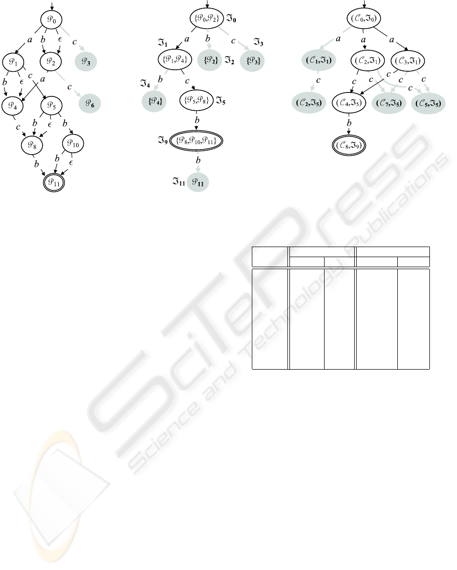
Figure 7: Lazy generation of Psp.O/ (left), Is p.O/ (center), and Bhv.}.˙ // (right).
late into Bhv.}.˙// as the new transition
.C
4
; =
5
/
b
! .C
8
; =
9
/, with the creation of
.C
8
; =
9
/. No inconsistent transition is detected.
Instead, u nlike the previous steps, at this point
the pruning of Bhv.}.˙// applies. We have
B
D B B
0
D f.C
2
; =
5
/; .C
7
; =
5
/; .C
5
; =
5
/g.
Since no transition exits either of these three
states and =
5
is not final in Isp.O/, these states
are removed from Bhv.}.˙//, alon g with en-
tering transitions. This provokes the removal of
state .C
1
; =
1
/ and its entering transition, too.
4. The last layer of Psp.O// is generated, involving
the final state P
11
and three entering transitio ns.
These causes the extension of Isp.O/ by Ext.=
9
/
and New.=
9
b
! =
11
/. However, the latter is in-
consistent in Bhv.}.˙//, therefore it is removed
from I sp.O/.
Compared with Fig. 4, t he number of states and
transitions in both Psp.O/ and Isp.O/ is reduced in
Fig. 7, as expected. Of course, the advantage in us-
ing the lazy approach depends on the extent of the set
resulting from the difference between the language
of Isp.O/ and the language of Bsp.˙;
0
/, in o ther
words, on the number of spurious traces in kOk: the
larger the set of spurious traces, the better the perfor-
mances of LDE compared with the busy approach.
5 EXPERIMENTAL RESULTS
The implementation of a prototype software sys-
tem, coded in the Haskell programming language
(Thompson, 1999), that embodies the lazy diagno-
sis method dealt with in this paper, was performed,
as well as the implementation of the (busy) diagnosis
method previously pr oposed for a-posteriori diagno-
sis (Lamperti and Zanella, 2003 ), the Diagnostic En-
gine (DE). As explained in Secti on 3, DE involves
no circular pruning. R at her, it pr ocesses in one step
the whole observation, in order to obtain the prefix
space. Then, it invokes the Subset Construction algo-
rithm (Hop croft et al., 2006) to determinize the whole
prefix space into the (whole) index space. Next, it
performs a reconstruction of the behavior driven by
the index space and, finally, it decorates the behavior
in or der to draw candidate diagnoses. Also the im-
plemented LDE, after having reconstructed the con -
densed behavior corresponding t o the whole observa-
tion, decorates it and draws candidate diagno ses.
In order to compare the performances of LDE and
DE, hundreds of experiments were run based on ob-
servations with different sizes and different overlays
between their extensions and the language of the be-
havior space. Such experiments have confirmed that
the savings in memory allocation b rought by LDE, as
far as the prefix space and the index space are con-
cerned, i ncrease with the size of the observation and,
given the same observation, decrease wi th the grow-
ing of the extent of the overl ay. Interestingly, the exe-
cution time of LDE was shorter than that of DE in all
experiments, with a saving in time having t he same
trend as the saving in space.
Shown in Table 1 are the size of the memor y al-
location and the execution time of the two methods,
corresponding to the number of nodes in the involved
observations. Memory allocation (space) is the max-
Figure 7: Lazy generation of Psp(O) (left), Isp(O) (center), and Bhv(℘(Σ)) (right).
5 EXPERIMENTAL RESULTS
The implementation of a prototype software system,
coded in the Haskell programming language (Thomp-
son, 1999), that embodies the lazy diagnosis method
dealt with in this paper, was performed, as well as the
implementation of the (busy) diagnosis method pre-
viously proposed for a-posteriori diagnosis (Lamperti
and Zanella, 2003), the Diagnostic Engine (DE). As
explained in Section 3, DE involves no circular prun-
ing. Rather, it processes in one step the whole obser-
vation, in order to obtain the prefix space. Then, it
invokes the Subset Construction algorithm (Hopcroft
et al., 2006) to determinize the whole prefix space into
the (whole) index space. Next, it performs a recon-
struction of the behavior driven by the index space
and, finally, it decorates the behavior in order to draw
candidate diagnoses. Also the implemented LDE, af-
ter having reconstructed the condensed behavior cor-
responding to the whole observation, decorates it and
draws candidate diagnoses.
In order to compare the performances of LDE and
DE, hundreds of experiments were run based on ob-
servations with different sizes and different overlays
between their extensions and the language of the be-
havior space. Such experiments have confirmed that
the savings in memory allocation brought by LDE, as
far as the prefix space and the index space are con-
cerned, increase with the size of the observation and,
given the same observation, decrease with the grow-
ing of the extent of the overlay. Interestingly, the exe-
cution time of LDE was shorter than that of DE in all
experiments, with a saving in time having the same
trend as the saving in space.
Table 1: LDE vs. DE
Space Time
Nodes DE LDE DE LDE
1 7 7 0.06 0.04
2 22 19 0.06 0.04
3 64 19 0.08 0.06
4 178 115 0.08 0.10
5 438 225 0.18 0.16
6 900 410 0.50 0.46
7 2286 931 4.70 1.30
8 5258 1976 39.84 3.94
9 10738 4093 293.60 10.90
10 20597 8476 1758.28 52.26
Shown in Table 1 are the size of the memory al-
location and the execution time of the two methods,
corresponding to the number of nodes in the involved
observations. Memory allocation (space) is the max-
imum value of the sum of nodes and arcs of both the
prefix space and the index space, while the execution
time is the CPU time in seconds. The table refers to
10 experiments led on a five-component seven-link
active system with totally disconnected observations
including from 1 to 10 nodes, where the observation
including n + 1 nodes is obtained by adding a new
node to the observation including n nodes (n ∈ [0 .. 9]).
6 CONCLUSIONS
This paper presents a lazy approach to diagnosis of
active systems with uncertain observations. It pri-
marily aims to reduce the size of the memory space
needed by the indexing automata for observation han-
dling. The lazy generation of the index space has been
DIAGNOSIS OF ACTIVE SYSTEMS BY LAZY TECHNIQUES
179

obtained by adapting an algorithm for incremental de-
terminization (Lamperti et al., 2008), by specializing
it to cope with acyclic automata. Experimental evi-
dence supports the theoretical claim of space reduc-
tion, and shows also a saving in computation time.
Pruning an uncertain observation based on an in-
cremental history reconstruction can be generalized to
domains other than active systems. The task of trans-
forming an uncertain observation graph into an au-
tomaton is not faced in (Grastien et al., 2005), where
it is assumed that the uncertain observation is rep-
resented by an automaton from the very beginning.
However, such an automaton could be pruned based
on a lazy technique similar to ours.
Other approaches in the literature have tried to im-
prove efficiency, above all for carrying out the mon-
itoring task, for which real time constraints hold, in-
cluding (Qiu and Kumar, 2006), whose computational
effort is linear. However, such an approach consid-
ers certain observations only and, at the moment, we
cannot devise how much the degrees as well as the
kinds of uncertainties that may affect an observation
can change such figures.
REFERENCES
Baroni, P., Lamperti, G., Pogliano, P., and Zanella, M.
(1998). Diagnosis of active systems. In Thir-
teenth European Conference on Artificial Intelligence
– ECAI’98, pages 274–278, Brighton, UK.
Baroni, P., Lamperti, G., Pogliano, P., and Zanella, M.
(1999). Diagnosis of large active systems. Artificial
Intelligence, 110(1):135–183.
Grastien, A., Cordier, M., and Largou
¨
et, C. (2005). Incre-
mental diagnosis of discrete-event systems. In Six-
teenth International Workshop on Principles of Diag-
nosis – DX’05, pages 119–124, Monterey, CA.
Hopcroft, J., Motwani, R., and Ullman, J. (2006). Introduc-
tion to Automata Theory, Languages, and Computa-
tion. Addison-Wesley, Reading, MA, third edition.
Lamperti, G. and Zanella, M. (2002). Diagnosis of discrete-
event systems from uncertain temporal observations.
Artificial Intelligence, 137(1–2):91–163.
Lamperti, G. and Zanella, M. (2003). Diagnosis of Active
Systems – Principles and Techniques, volume 741 of
The Kluwer International Series in Engineering and
Computer Science. Kluwer Academic Publisher, Dor-
drecht, NL.
Lamperti, G. and Zanella, M. (2004). A bridged diagnostic
method for the monitoring of polymorphic discrete-
event systems. IEEE Transactions on Systems, Man,
and Cybernetics – Part B: Cybernetics, 34(5):2222–
2244.
Lamperti, G. and Zanella, M. (2006). Flexible diagnosis of
discrete-event systems by similarity-based reasoning
techniques. Artificial Intelligence, 170(3):232–297.
Lamperti, G. and Zanella, M. (2008). Observation-
subsumption checking in similarity-based diagnosis
of discrete-event systems. In Eighteenth European
Conference on Artificial Intelligence – ECAI’2008,
pages 204–208, Patras, G.
Lamperti, G., Zanella, M., Chiodi, G., and Chiodi, L.
(2008). Incremental determinization of finite au-
tomata in model-based diagnosis of active systems.
In Lovrek, I., Howlett, R., and Jain, L., editors,
Knowledge-Based Intelligent Information and Engi-
neering Systems, volume 5177 of LNAI, pages 362–
374. Springer.
Pencol
´
e, Y. and Cordier, M. (2005). A formal framework
for the decentralized diagnosis of large scale discrete
event systems and its application to telecommunica-
tion networks. Artificial Intelligence, 164:121–170.
Qiu, W. and Kumar, R. (2006). Decentralized failure diag-
nosis of discrete event systems. IEEE Transactions on
Systems, Man, and Cybernetics – Part A: Systems and
Humans, 36(2):384–395.
Sampath, M., Sengupta, R., Lafortune, S., Sinnamohideen,
K., and Teneketzis, D. (1995). Diagnosability of
discrete-event systems. IEEE Transactions on Auto-
matic Control, 40(9):1555–1575.
Sampath, M., Sengupta, R., Lafortune, S., Sinnamohideen,
K., and Teneketzis, D. (1996). Failure diagnosis using
discrete-event models. IEEE Transactions on Control
Systems Technology, 4(2):105–124.
Thompson, S. (1999). Haskell – The Craft of Functional
Programming. Addison-Wesley, Harlow, UK.
ICEIS 2010 - 12th International Conference on Enterprise Information Systems
180
