IMPROVEMENT OF DIFFERENTIAL CRISP CLUSTERING USING

ANN CLASSIFIER FOR UNSUPERVISED PIXEL

CLASSIFICATION OF SATELLITE IMAGE

Indrajit Saha, Dariusz Plewczynski

ICM, University of Warsaw, 02-089 Warsaw, Poland

Ujjwal Maulik

Department of Computer Science and Engineering, Jadavpur University, Kolkata-700032, West Bengal, India

Sanghamitra Bandyopadhyay

Machine Intelligence Unit, Indian Statistical Institute, Kolkata-700108, West Bengal, India

Keywords:

ANN classiﬁer, Crisp clustering, Differential evolution, Statistical signiﬁcance test, IRS satellite image.

Abstract:

An important approach to unsupervised pixel classiﬁcation in remote sensing satellite imagery is to use clus-

tering in the spectral domain. In particular, satellite images contain landcover types some of which cover

signiﬁcantly large areas, while some (e.g., bridges and roads) occupy relatively much smaller regions. De-

tecting regions or clusters of such widely varying sizes presents a challenging task. This fact motivated us to

present a novel approach that integrates a differential evaluation based crisp clustering scheme with artiﬁcial

neural networks (ANN) based probabilistic classiﬁer to yield better performance. Real-coded encoding of the

cluster centres is used for the differential evaluation based crisp clustering. The clustered solution is then used

to ﬁnd some points based on their proximity to the respective centres. The ANN classiﬁer is thereafter trained

by these points. Finally, the remaining points are classiﬁed using the trained classiﬁer. Results demonstrating

the effectiveness of the proposed technique are provided for several synthetic and real life data sets. Also sta-

tistical signiﬁcance test has been performed to establish the superiority of the proposed technique. Moreover,

one remotely sensed image of Bombay city has been classiﬁed using the proposed technique to establish its

utility.

1 INTRODUCTION

For remote sensing applications, classiﬁcation is an

important task which partitions the pixels in the im-

ages into homogeneous regions, each of which corre-

sponds to some particular landcover type. The prob-

lem of pixel classiﬁcation is often posed as clustering

in the intensity space. In a satellite image, each pixel

represents a landcover area, which may not necessar-

ily belong to a single landcover type. Thus in remote

sensing images, large number of pixels may have sig-

niﬁcant belongingness to multiple classes. There-

fore a large amount of uncertainty is associated with

the pixels in a remotely sensed image. In the unsu-

pervised pixel classiﬁcation framework, various clus-

tering algorithms like K-means (Everitt, 1993; Jain

et al., 1999), split-and-merge (Laprade, 1988) and

scale space techniques (Wong and Posner, 1993) have

been used for the purpose of satellite image segmen-

tation.

Clustering (Jain and Dubes, 1988) is a useful unsu-

pervised data mining technique which partitions the

input space into K regions depending on some simi-

larity/dissimilarity metric where the value of K may

or may not be known a priori. K-means (Jain et al.,

1999) is a traditional partitional clustering algorithm

which starts with K random cluster centroids and the

centroids are updated in successive iterations by com-

puting the numerical averages of the feature vectors in

each cluster. The objective of the K-means algorithm

is to maximize the global compactness of the clusters.

The main disadvantages of the K-means clustering al-

Saha I., Plewczynski D., Maulik U. and Bandyopadhyay S. (2010).

IMPROVEMENT OF DIFFERENTIAL CRISP CLUSTERING USING ANN CLASSIFIER FOR UNSUPERVISED PIXEL CLASSIFICATION OF

SATELLITE IMAGE.

In Proceedings of the 12th International Conference on Enterprise Information Systems - Artiﬁcial Intelligence and Decision Support Systems, pages

21-29

DOI: 10.5220/0002872800210029

 SciTePress

gorithm are (1) it depends much on the initial choice

of the modes and (2) it often gets trapped into some

local optimum. However, these facts are motivated us

to provide a new crisp clustering technique and it’s

improvement using supervised classiﬁer.

In 1995 a new ﬂoating point encoded evolutionary

algorithm for global optimization called Differential

Evolution (DE) was proposed in (Storn and Price,

1997) that uses a special kind of differential opera-

tor. Recently, DE has been found a wide spread ap-

plication in different ﬁelds of engineering and sci-

ence. Also by carrying this fact, we are propos-

ing a integrated approach with differential evaluation

based crisp clustering (DECC) and ANN classiﬁer

(Bishop, 1996; MacKay, 1992). The differential eval-

uation based crisp clustering technique is used to ﬁnd

the proper partitions and after that, the ANN clas-

siﬁer is trained by fraction of data points, selected

based on their proximity to the respective centres. Fi-

nally, remaining points are classiﬁed by trained clas-

siﬁer. The efﬁciency of the proposed technique is

compared with genetic algorithm based crisp cluster-

ing (GACC), simulated annealing based crisp clus-

tering (SAFC) and well-known K-mean (Jain et al.,

1999) algorithm. However, it’s integrated version like

GACC-ANN, SACC-ANN and K-means-ANN has

also been tested. Effectiveness of this proposed tech-

nique has been established by quantitatively, visually

and statistically. Moreover, Different landcover re-

gions in remote sensing imagery have also been clas-

siﬁed using the proposed technique.

2 CRISP CLUSTERING

ALGORITHMS

2.1 K-means

The K-means algorithm (Jain et al., 1999), one of the

most widely used ones, attempts to solve the cluster-

ing problem by optimizing a given metric. The objec-

tive to minimize the within cluster variance ζ.

ζ =

∑

i=1

∑

x∈C

D(x, m

) (1)

Here m

is the mean of clusterC

and D(x, m

) denotes

the distance between the point x and m

. K denotes

the number of clusters. The resulting clustering of the

data set X is usually only a local minimum of ζ. The

idea in K-means is to select K representativepoints as

a centre, in X and assign the rest of the data points to

the cluster identiﬁed by the nearest. Initial set of K

centres are selected randomly. Subsequently, all the

points in X are assigned to the nearest centre. In each

iteration, a new mean is determined for each cluster.

After that, all the points in X are reassigned to their

clusters in accordance with the new set of centre or

mean. The algorithm iterates until ζ does not change

any more.

2.2 Genetic Algorithm based Crisp

Clustering

In Genetic Algorithm (Goldberg, 1989) based Crisp

Clustering (GACC), the chromosomes are made up of

real numbers which represent the coordinates of the

centres of the partitions. If chromosome i encodes the

centres of K clusters in d dimensional space then its

length l is d × K. For initializing a chromosome, the

K centres are randomly selected points from the data

set while ensuring that they are distinct. The ﬁtness

of a chromosome indicates the degree of goodness of

the solution it represents. In this article, ζ is used for

this purpose. The objective is therefore to minimize

ζ for achieving proper clustering. Given a chromo-

some, the centres encoded in it are ﬁrst extracted. Let

the chromosome encode K centres, and let these be

denoted as z

, z

, . . . , z

. The centres encoded in a

chromosome are updated new set of centres or mean.

Conventional proportional selection implemented by

the roulette wheel strategy is applied on the popula-

tion of strings. The standard single point crossover is

applied stochastically with probability µ

. The clus-

ter centres are considered to be indivisible, i.e., the

crossover points can only lie in between two clusters

centres. In each gene position of a chromosome is

subjected to mutation with a ﬁxed probability µ

, re-

sulting in the overall perturbation of the chromosome.

A number ± in the range [0, 1] is generated with uni-

form distribution. If the value at a gene position is v,

after mutation it becomes (1±2×δ)×v, when v 6= 0,

and ±2×δ, when v = 0. The ’+’ or ’-’ sign occurs

with equal probability. Note that, because of muta-

tion more than one cluster centre may be perturbed in

a chromosome. The algorithm is termination after it

has executed a ﬁxed number of generations. The eli-

tist model of GAs has been used, where the best string

seen so far is stored in a location within the popula-

tion. The best string of the last generation provides

the solution to the clustering problem. Fig. 1 demon-

strate the GACC algorithm.

2.3 Simulated Annealing based Crisp

Clustering

Simulated annealing (SA) (Kirkpatrik et al., 1983;

van Laarhoven and Aarts, 1987) is an optimization

ICEIS 2010 - 12th International Conference on Enterprise Information Systems

Initial Population.

(Here each chromosome encodes real value of corre-

sponding to K centres)

Fitness computation using ζ. (see Eqn. (1))

Repeat

Roulette Wheel Selection.

Crossover.

Mutation.

Fitness Computation.

Until (termination criteria are met)

Figure 1: GACC Algorithm.

tool which has successful applications in a wide range

of combinatorial as well as functional optimization

problems. The fact motivated researchers to use a SA

to optimize the clustering problem where it provides

near optimal solutions of an objective or ﬁtness func-

tion in complex, large and multimodal landscapes. In

Simulated Annealing based Crisp Clustering (SACC)

a string or conﬁguration encodes d × K cluster cen-

tres. Subsequently the string is updated using the new

centres, computed as a mean. Thereafter the energy

function, ζ, is computed as per Eqn. (1). The cur-

rent string is perturbed using the mutation operation

as discussed for GACC. This way, perturbation of a

string yields a new string. It’s energy is also computed

in a similar fashion. If the energy of the new string

(E(s)) is less than that of the current string (E(p)), the

new string is accepted. Otherwise the newstring is ac-

cepted based on a probability

exp(−(E(s)−E(p)))

where

T is the current temperature of the SA process. Fig. 2

describes the SACC algorithm in detail.

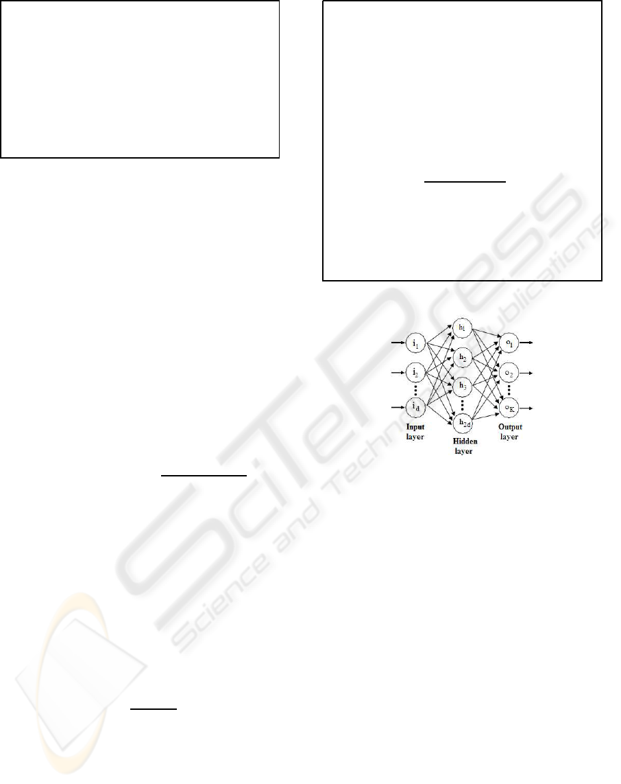
3 ANN BASED CLASSIFIER

The ANN classiﬁer (Fig. 3) algorithm used in this

article implements a three layer feed-forward neu-

ral network with a hyperbolic tangent function for

the hidden layer and the softmax function (Andersen

et al., 1997) for the out put layer. Using softmax, out-

put of ith output neuron is given by:

∑

j=1

(2)

where q

the net input to the ith output neuron, and K

is the number of output neurons. The use of softmax

makes it possible to interpret the outputs as probabil-

ities. The number of neurons in the input layer is d,

where d is the number of features of the input data

set. The number of neurons in the output layer is

K, where K is the number of classes. The ith out-

put neuron provides the class membership degree of

p = Random initial conﬁguration.

(Here each chromosome encodes real value of corre-

sponding to K centres)

T = T

max

E(p) = Energy of p is computed using Eqn. (1).

while( T ≥ T

min

)

for i = 1 to k

s = Perturb ( p ).

E(s) = Energy of s is computed using Eqn. (1).

if (E(s) - E(p) < 0 )

Set p = s and E(p) = E(s)

else

if (rand(0,1) <

exp(−(E(s)−E(p)))

)

Set p = s and E(p) = E(s)

end if

end for

T= T×r. /* 0 < r < 1 */

end while

Figure 2: SACC Algorithm.

Figure 3: Three layer feed-forward ANN classiﬁer model.

the input pattern to the ith class. The number of hid-

den layer neurons is taken as 2× d. The weights are

optimized with a maximum a posteriori (MAP) ap-

proach; cross-entropy error function augmented with

a Gaussian prior over the weights. The regularization

is determined by MacKay’s ML-II scheme (MacKay,

1992). Outlier probability of training examples is also

estimated (Sigurdsson et al., 2002). Fig. 3 shows the

feed-forward ANN classiﬁer model.

4 PROPOSED TECHNIQUE

4.1 Differential Evolution based Crisp

Clustering

Differential Evolution (Storn and Price, 1995; Storn

and Price, 1997) is a relatively recent heuristic de-

signed to optimize problems over continuous do-

mains. In DECC, Each vector is a sequence of real

numbers representing the K cluster centres. For an d-

dimensional space, the length of a vector is l = d × K,

IMPROVEMENT OF DIFFERENTIAL CRISP CLUSTERING USING ANN CLASSIFIER FOR UNSUPERVISED

PIXEL CLASSIFICATION OF SATELLITE IMAGE

where the ﬁrst d positions represent the ﬁrst cluster

centre, the next d positions represent those of the sec-

ond cluster centre, and so on. The K cluster centres

encoded in each vector are initialized to K randomly

chosen points from the data set. This process is re-

peated for each of the P vectors in the population,

where P is the size of the population. The kth individ-

ual vector of the population at time-step (generation)

t has l components (d × K), i.e.,

(t) = [G

k,1

(t), G

k,2

(t), . . . , G

k,l

(t)] (3)

For each target vector G

(t) that belongs to the cur-

rent population, three randomly selected vectors from

the current population is used. In other words the lth

component of each trial offspring is generated as fol-

lows.

(t + 1) = G

(t) + F (G

(t) − G

(t)) (4)

Here F is a mutation factor. In order to increase

the diversity of the perturbed parameter vectors,

crossover is introduced. To this end, the trial vector:

(t + 1) = [Q

k,1

(t + 1), Q

k,2

(t + 1), . . . , Q

k,l

(t + 1)]

(5)

is formed, where

(t+1) =











(t + 1)

if rand

(0, 1) ≤ CR or j = rand(k)

(t)

if rand

(0, 1) > CR and j 6= rand(k)

(6)

In Eqn. (6), rand

(0, 1) is the jth evaluation of a uni-

form random number generator with outcome ∈ [0,

1]. CR is the crossover rate ∈ [0, 1] which has to be

determined by the user. rand(k) is a randomly chosen

index ∈ {1, 2,. . .,d} which ensures that Q

(t + 1) gets

at least one parameter from ϑ

(t + 1). The following

condition decide whether or not it should become a

member of next generation (t + 1),

(t + 1) =











(t + 1)

if f(Q

(t + 1)) > f(G

)

(t)

if f(Q

(t + 1)) ≤ f(G

)

(7)

where f(.) is the objective function to be minimized

in this article. The processes of mutation, crossover

and selection are executed for a ﬁxed number of iter-

ations. The best vector seen up to the last generation

provides the solution to the clustering problem.

4.2 Integration with ANN Classiﬁer

Step1: After execution of DECC or GACC or SACC

or K-means to obtain a best solution vector

consisting of cluster centres.

Step2: Select 50% of data points from each clus-

ter which are nearest to the respective cluster

centres. The class labels of the points are set

to the respective cluster number.

Step3: Train a ANN classiﬁer with the points se-

lected in step 2.

Step4: Generate the class labels for the remaining

points using the trained ANN classiﬁer.

5 EXPERIMENTAL RESULTS

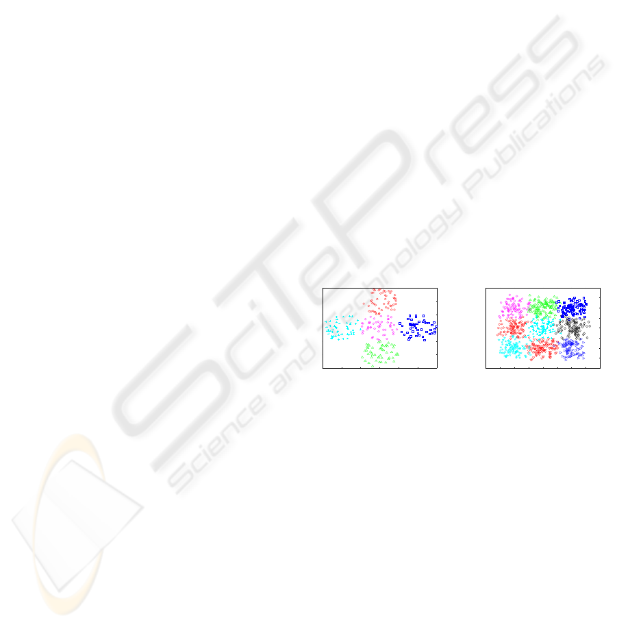
5.1 Artiﬁcial Data Sets

Data1: This is an overlapping two dimensional data

set where the number of clusters is ﬁve. It has 250

points. The value of K is chosen to be 5. The data set

is shown in Fig. 4.a.

Data2: This is also a two dimensional data set con-

sisting of 900 points. The data set has 9 classes. The

data set is shown in Fig. 4.b.

4 6 8 10 12 14 16

−4 −3 −2 −1 0 1 2 3 4

−4

−3

−2

−1

(a) (b)

Figure 4: Two Artiﬁcial Data Set (a) and (b).

5.2 Real-life Data Sets

Iris: This data consists of 150 patterns divided into

three classes of Iris ﬂowers namely, Setosa, Virginia

and Versicolor. The data is in four dimensional space

(sepal length, sepal width, petal length and petal

width).

Cancer: It has 683 patterns in nine features (clump

thickness, cell size uniformity, cell shape uniformity,

marginal adhesion, single epithelial cell size, bare nu-

clei, bland chromatin, normal nucleoli and mitoses),

and two classes malignant and benign. The two

classes are known to be linearly inseparable.

ICEIS 2010 - 12th International Conference on Enterprise Information Systems

5.3 Performance Metrics

5.3.1 Minkowski Score

The performances of the clustering algorithms are

evaluated in terms of the Minkowski Score (MS) (Jar-

dine and Sibson, 1971). This is a measure of the qual-

ity of a solution given the true clustering. Let T be

the “true” solution and S the solution we wish to mea-

sure. Denote by n

the number of pairs of elements

that are in the same cluster in both S and T. Denote

by n

the number of pairs that are in the same cluster

only in S, and by n

the number of pairs that are in

the same cluster in T. Minkowski Score (MS) is then

deﬁned as:

MS =

+ n

(8)

For MS, the optimum score is 0, with lower scores

being “better”.

5.4 Input Parameters

The population size and number of generation used

for DECC and GACC are 50 and 100 respectively.

The crossoverprobability and mutation factors (F) for

DECC are set to be 0.8 and 0.7, respectively. The

crossover and mutation probabilities for GACC are

taken to be 0.8 and 0.3, respectively. The parame-

ters of the SA based fuzzy clustering algorithm are as

follows: T

max

=100, T

min

=0.01, r=0.9 and k=100. The

K-means algorithm is executed till it converges to the

ﬁnal solution. For all the fuzzy clustering algorithms

m, the fuzzy exponent, is set to 2.0. Results reported

in the tables are the average values obtained over 50

runs of the algorithms. Note that the input parame-

ters used here are ﬁxed either following the literature

or experimentally. For example the value of fuzzy

exponent (m), the scheduling of simulated annealing

follows the literature whereas the crossover, mutation

probability, population size, number of generation is

ﬁxed experimentally.

5.5 Performance

Tables 1 to 2 report the average values of ζ and

MS indices provided by DECC-ANN, GACC-ANN,

SACC-ANN, K-means-ANN, DECC, GACC, SACC

and K-means clustering over 50 runs of the algo-

rithms for the two synthetic and two real life data

sets considered here. The values reported in the

tables show that for all the data sets, DECC-ANN

provides the best ζ and MS indices score. For ex-

ample, Cancer data set, the average value of MS

produces by DECC-ANN algorithm is 0.3511. The

MS value produce by GACC-ANN, SACC-ANN, K-

means-ANN, DECC, GACC, SACC and K-means are

0.3702, 0.3873, 0.4502, 0.3733, 0.3839, 3945 and

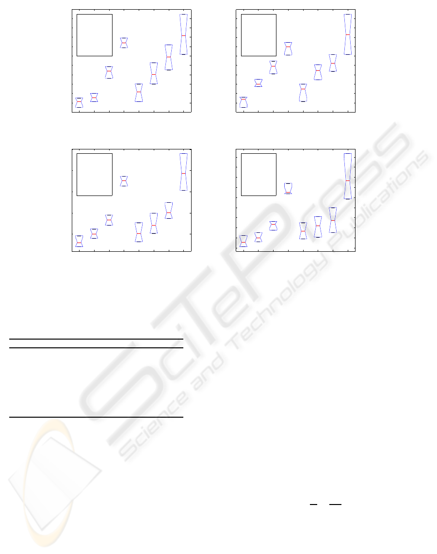
0.4733, respectively. Fig. 5 demonstrates the box-

plot as well as the convergence plot of different al-

gorithms. As can be seen from the ﬁgures the perfor-

mance of the proposed DECC-ANN is the best for all

the data sets.

Table 1: Average ζ and MS values over 50 runs of different

algorithms for the two Artiﬁcial data sets.

Algorithms Data1 Data1

ζ MS ζ MS

DECC-ANN 486.17 0.3022 467.33 0.4074

GACC-ANN 488.34 0.3108 470.62 0.4404

SACC-ANN 490.71 0.3673 475.53 0.4784

K-means-ANN 496.72 0.4283 481.64 0.5194

DECC 488.02 0.3231 469.05 0.4293

GACC 489.16 0.3604 472.5 0.4694

SACC 494.65 0.3982 477.47 0.4844

K-means 498.36 0.4433 484.88 0.5454

Table 2: Average ζ and MS values over 50 runs of different

algorithms for the two Real-life data sets.

Algorithms Iris Cancer

ζ MS ζ MS

DECC-ANN 75.05 0.3803 19324.13 0.3511

GACC-ANN 77.62 0.4004 19327.04 0.3702

SACC-ANN 80.72 0.4336 193330.62 0.3873

K-means-ANN 83.07 0.5257 19336.82 0.4502

DECC 78.93 0.4013 19327.54 0.3733

GACC 79.83 0.4210 19329.02 0.3839

SACC 82.62 0.4502 19332.42 0.3945

K-means 85.42 0.5434 19339.82 0.4733

5.6 Statistical Signiﬁcance Test

A non-parametric statistical signiﬁcance test called

Wilcoxons rank sum test (Hollander and Wolfe, 1999)

for independent samples has been conducted at the

5% signiﬁcance level. Eight groups, corresponding

to the eight algorithms (1. DECC-ANN, 2. GACC-

ANN, 3. SACC-ANN, 4. K-means-ANN, 5. DECC,

6. GACC, 7. SACC, 8. K-means), have been created

for each data set. Each group consists of the MS for

the data sets produced by 50 consecutive runs of the

corresponding algorithm. The median values of each

group for all the data sets are shown in Table 3.

It is evident from Table 3 that the median values

for DECC-ANN are better than that for other algo-

rithms. To establish that this goodness is statisti-

cally signiﬁcant, Table 4 reports the p-values pro-

duced by Wilcoxons rank sum test for comparison

of two groups (one group corresponding to DECC-

ANN and another group corresponding to some other

algorithm) at a time. As a null hypothesis, it is as-

sumed that there is no signiﬁcant difference between

the median values of two groups. Whereas, according

to the alternative hypothesis there is signiﬁcant differ-

IMPROVEMENT OF DIFFERENTIAL CRISP CLUSTERING USING ANN CLASSIFIER FOR UNSUPERVISED

PIXEL CLASSIFICATION OF SATELLITE IMAGE

1 2 3 4 5 6 7 8

0.3

0.32

0.34

0.36

0.38

0.4

0.42

0.44

0.46

0.48

Minkowski Score

Different Algorithms

1−>DECC−ANN

2−>GACC−ANN

3−>SACC−ANN

4−>K−means−ANN

5−>DECC

6−>GACC

7−>SACC

8−>K−means

1 2 3 4 5 6 7 8

0.4

0.42

0.44

0.46

0.48

0.5

0.52

0.54

0.56

0.58

Minkowski Score

Different Algorithms

1−>DECC−ANN

2−>GACC−ANN

3−>SACC−ANN

4−>K−means−ANN

5−>DECC

6−>GACC

7−>SACC

8−>K−means

(a) (b)

1 2 3 4 5 6 7 8

0.4

0.45

0.5

0.55

0.6

Minkowski Score

Different Algorithms

1−>DECC−ANN

2−>GACC−ANN

3−>SACC−ANN

4−>K−means−ANN

5−>DECC

6−>GACC

7−>SACC

8−>K−means

1 2 3 4 5 6 7 8

0.34

0.36

0.38

0.4

0.42

0.44

0.46

0.48

0.5

0.52

Minkowski Score

Different Algorithms

1−>DECC−ANN

2−>GACC−ANN

3−>SACC−ANN

4−>K−means−ANN

5−>DECC

6−>GACC

7−>SACC

8−>K−means

Figure 5: Boxplot of MS for different clustering algorithms for (a) Data1, (b) Data2, (c) Iris and (d) Cancer data sets.

Table 3: Median values of the Minkowski Scores for the

Data sets over 50 consecutive runs of different algorithms.

Algorithm Data1 Data2 Iris Cancer

DECC-ANN 0.2946 0.4122 0.3982 0.3483

GACC-ANN 0.3203 0.4582 0.4144 0.3872

SACC-ANN 0.3503 0.4673 0.4283 0.3953

K-means-ANN 0.4377 0.5244 0.5382 0.4483

DECC 0.3352 0.4261 0.4102 0.3672

GACC 0.3572 0.4577 0.4601 0.3903

SACC 0.3862 0.4902 04682 0.4035

K-means 0.4521 0.5563 0.5482 0.4837

ence in the median values of the two groups. All the

p-values reported in the table are less than 0.05 (5%

signiﬁcance level). For example, the rank sum test

between the algorithms DECC-ANN and GACC for

Iris provides a p-value of 1.3253e-004, which is very

small. This is strong evidence against the null hypoth-

esis, indicating that the better median values of the

performance metrics produced by DECC-ANN is sta-

tistically signiﬁcant and has not occurred by chance.

Similar results are obtained for all other data sets and

for all other algorithms compared to DECC-ANN, es-

tablishing the signiﬁcant superiority of the proposed

technique.

6 APPLICATION TO SATELLITE

IMAGE SEGMENTATION

In this section, an IRS remote sensing satellite im-

age of a part of the city of Bombay has been used for

demonstrating unsupervised pixel classiﬁcation. The

results obtained by application of DECC-ANN clus-

tering have been reported and compared with other

stated clustering algorithms. The results are shown

both graphically and numerically. To show the effec-

tiveness of the DECC-ANN technique, a cluster va-

lidity index I (Maulik and Bandyopadhyay,2002) has

been examined. The index I , proposed recently as a

measure of indicating the goodness/validity of cluster

solution, is deﬁned as follows:

I (K) = (

× D

)

, (9)

where K is the number of clusters. Here,

∑

k=1

∑

i=1

k,i

k z

− x

k, (10)

and

= max

k6= j

k z

− z

k, (11)

In this article, we have taken p = 2. Here u

k,i

is the

ICEIS 2010 - 12th International Conference on Enterprise Information Systems

Table 4: P− values produced by Wilcoxon’s Rank Sum test comparing with DECC-ANN with other algorithms.

DataSet P-value

GACC-ANN SACC-ANN K-means-ANN DECC GACC SACC K-means

Data1 0.0302 2.0361e-003 1.4077e-004 0.0125 1.6327e-004 3.8224e-004 5.3075e-005

Data2 0.0313 2.8531e-003 .2934e-004 0.0173 1.3253e-004 4.0504e-004 4.9177e-005

Iris 0.03150 3.6603e-003 2086e-004 0.0162 1.3253e-004 3.9204e-004 4.8177e-005

Cancer 0.031 2.0462e-003 1.2086e-004 0.0147 1.3586e-004 4.3858e-004 4.9177e-005

City

Area

Islands

The

Dockyard

Island

The

Arabian

Sea

Figure 6: IRS image of Bombay in the NIR band with his-

togram equalization.

membership of pattern x

to the kth cluster. For crisp

clustering u

k,i

will be 0 or 1. Larger value of I index

implies better solution.

Note that for computing the Minkowski score, knowl-

edge about the true partitioning of the data is neces-

sary. This knowledge is not available for the pixel

classiﬁcation problem considered here. Therefore, the

Minkowski Score can not be used for evaluating clus-

tering performance in this case. Hence the internal

clustering criterion I index is used for performance

comparison. Larger value of I index implies a better

solution.

6.1 IRS Image of Bombay

The data used here was acquired from the Indian

Remote Sensing Satellite (IRS-1A) (irs, 1986) us-

ing the LISS-II sensor that has a resolution of

36.25m×36.25m. The image is contained in four

spectral bands namely, blue band of wavelength 0.45-

0.52 µm, green band of wavelength 0.52-0.59 µm, red

band of wavelength 0.62-0.68 µm, and near infra red

band of wavelength 0.77-0.86 µm. Each band is of

size 512 × 512, i.e., the size of the data set to be clus-

tered in all the bands is 262144.

Fig. 6 shows the IRS image of a part of Bombay in

the near infrared band. As can be seen, the city area is

enclosed on three sides by the Arabian sea. Towards

Figure 7: Clustered IRS image of Bombay using DECC-

ANN technique.

the bottom right of the image, there are many islands,

including the famous Elephanta island. The dockyard

is situated on the south eastern part of Bombay, which

can be seen as a set of three ﬁnger like structure. As

per our ground knowledge, these clusters correspond

to 7 landcoverregions namely concrete (Concr.), open

spaces (OS1 and OS2), vegetation (Veg), habitation

(Hab), and turbid water (TW1 and TW2).

The result of the application of the proposed

DECC-ANN technique on the Bombay image is

shown in Fig. 7. The southern part of the city, which

is heavily industrialized, has been classiﬁed as pri-

marily belonging to habitation and concrete. Here,

the class habitation represents the regions having

concrete structures and buildings, but with relatively

lower density than the class Concrete. Hence these

two classes share common properties. From the re-

sult, it appears that the large water body of Arabian

sea is grouped into two classes (TW1 and TW2). It is

evident from the ﬁgure that the sea water has two dis-

tinct regions with different spectral properties. Hence

the clustering result providing two partitions for this

region is quite expected. Most of the islands, dock-

yard, several road structures have been correctly iden-

tiﬁed in the image. As expected, there is a high pro-

portion of open space and vegetation within the is-

lands.

Fig. 8 demonstrates the Bombay image clustered

using the GACC-ANN clustering algorithm. It can be

IMPROVEMENT OF DIFFERENTIAL CRISP CLUSTERING USING ANN CLASSIFIER FOR UNSUPERVISED

PIXEL CLASSIFICATION OF SATELLITE IMAGE

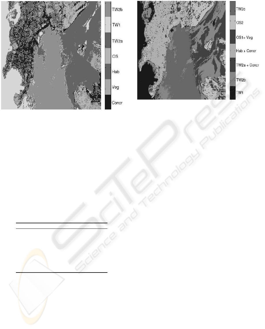
Figure 8: Clustered IRS image of Bombay using GACC-

ANN technique.

noted from the ﬁgure that the water of the Arabian sea

has been wrongly clustered into three regions, rather

than two as obtained earlier. It appears that the other

regions in the image have been classiﬁed more or less

correctly for this data. In Fig. 9, the Bombay image

clustered using K-means clustering has been shown.

It appears from the ﬁgure that the sea area is wrongly

classiﬁed into four different regions. Also there are

overlapping between the classes turbid water and con-

crete, as well as between open space and vegetation.

Table 5: Average ζ and MS values over 50 runs of different

algorithms for the two Real-life data sets.

Algorithms ζ I

DECC-ANN 3891147.3809 356.5182

GACC-ANN 3891234.7731 322.0861

SACC-ANN 3891361.5029 278.9641

K-means-ANN 3891607.8262 224.6372

DECC 3891206.4133 328.8802

GACC 3891295.8029 306.6037

SACC 3891422.8442 257.0382

K-means 3891791.0749 203.3929

The superiority of the DECC-ANN technique

can also be veriﬁed from the I index values that

are reported in Table 5. The ζ and I index val-

ues for DECC-ANN are tabulated along with other

algorithms. From the table, it is found for I

index that these values are 356.5182, 322.0861,

278.9641, 224.6372, 328.8802, 306.6037, 257.0382

and 203.3929, respectively. As a higher value of I

index indicates better clustering result, it follows that

DECC-ANN outperforms over the other algorithms.

Figure 9: Clustered IRS image of Bombay using K-means

algorithm.

7 CONCLUSIONS

This article proposes a newly developed integrated

clustering technique. The developed technique in-

tegrates differential evolution based crisp clustering

with ANN classiﬁer. The differential evolution based

crisp clustering technique minimize the intra cluster

compactness ζ for ﬁnding the proper partitions. Af-

ter that, the ANN classiﬁer is used to train by the

fraction of data points, selected based on their prox-

imity to the respective centres. Finally, remaining

points are thereafter classiﬁed by the trained classi-

ﬁer. For demonstrating the superiority of the tech-

nique, its performance has been compared with those

of genetic algorithm based crisp clustering, simulated

annealing based crisp clustering and K-means for two

synthetic and two real life data sets. It’s integrated

version has also been tested. Statistical signiﬁcance

test based on Wilcoxon’s rank sum test has been con-

ducted to judge the statistical signiﬁcance of the clus-

tering solutions produced by different algorithms. In

this context, IRS satellite image of Mumbai has been

classiﬁed using the proposed technique and compared

with other clustering algorithms. The results indicate

that the newly developed DECC-ANN technique can

be efﬁciently used for clustering different data sets.

As a scope of further research, performance of other

popular classiﬁers can be tested. The work can also

be extended to solve clustering problems where the

number of clusters is not known a priori. Finally, ap-

plication of DECC-ANN to several real life domains

e.g., VLSI system design, data mining and web min-

ing, needs to be demonstrated. The authors are cur-

rently working in this direction.

ICEIS 2010 - 12th International Conference on Enterprise Information Systems

ACKNOWLEDGEMENTS

This work was also supported by the Polish Ministry

of Education and Science (grants N301 159735, N518

409238, and others).

REFERENCES

(1986). IRS data users handbook. NRSA, Hyderabad, In-

dia.

Andersen, L. N., Larsen, J., Hansen, L. K., and HintzMad-

sen, M. (1997). Adaptive regularization of neural clas-

siﬁers. In. Proc. of the IEEE workshop on neural net-

works for signal processing VII, NewYork, USA, pages

24–33.

Bishop, C. (1996). Neural Networks for Pattern Recogni-

tion. Oxford University Press.

Everitt, B. S. (1993). Cluster Analysis. Halsted Press, Third

edition.

Goldberg, D. E. (1989). Genetic Algorithms in Search, Op-

timization and Machine Learning. Addison-Wesley,

New York.

Hollander, M. and Wolfe, D. A. (1999). Nonparametric

Statistical Methods. 2nd ed.

Jain, A. K. and Dubes, R. C. (1988). Algorithms for Clus-

tering Data. Prentice-Hall, Englewood Cliffs, NJ.

Jain, A. K., Murty, M. N., and Flynn, P. J. (1999). Data

clustering: A review, volume 31.

Jardine, N. and Sibson, R. (1971). Mathematical Taxonomy.

John Wiley and Sons.

Kirkpatrik, S., Gelatt, C. D., and Vecchi, M. P. (1983). Op-

timization by simulated annealing. Science, 220:671–

680.

Laprade, R. H. (1988). Split-and-merge segmentation of

aerial photographs. Computer Vision Graphics and

Image Processing, 48:77–86.

MacKay, D. J. C. (1992). The evidence framework ap-

plied to classiﬁcation networks. Neural Computation,

4:720–736.

Maulik, U. and Bandyopadhyay, S. (2002). Performance

evaluation of some clustering algorithms and validity

indices. IEEE Transactions on Pattern Analysis and

Machine Intelligence, 24(12):1650–1654.

Sigurdsson, S., Larsen, J., and Hansen, L. (2002). Out-

lier estimation and detection: application to skin le-

sion classiﬁcation. In Proc. Int. conf. on acoustics,

speech and signal processing.

Storn, R. and Price, K. (1995). Differential evolution - A

simple and efﬁcient adaptive scheme for global op-

timization over continuous spaces. Technical Report

TR-95-012, International Computer Science Institute,

Berkley (1995).

Storn, R. and Price, K. (1997). Differential evolution - A

simple and efﬁcient heuristic strategy for global opti-

mization over continuous spaces. Journal of Global

Optimization, 11:341–359.

van Laarhoven, P. J. M. and Aarts, E. H. L. (1987). Sim-

ulated Annealing: Theory and Applications. Kluwer

Academic Publisher.

Wong, Y. F. and Posner, E. C. (1993). A new clustering

algorithm applicable to polarimetric and sar images.

IEEE Transactions on Geoscience and Remote Sens-

ing, 31(3):634–644.

IMPROVEMENT OF DIFFERENTIAL CRISP CLUSTERING USING ANN CLASSIFIER FOR UNSUPERVISED

PIXEL CLASSIFICATION OF SATELLITE IMAGE