AUTONOMOUS MANEUVERS OF A FARM VEHICLE
WITH A TRAILED IMPLEMENT IN HEADLAND
Christophe Cariou, Roland Lenain, Michel Berducat
Cemagref, UR TSCF, 24 avenue des Landais, 63172 Aubi`ere, France
Benoit Thuilot
Clermont Universit´e, Universit´e Blaise Pascal, LASMEA, BP 10448, 63000 Clermont-Ferrand, France
Keywords:
Guidance system, Mobile robot, Path planning, Motion control, Agriculture.
Abstract:
This paper addresses the problem of path generation and motion control for the autonomous maneuvers of
a farm vehicle with a trailed implement in headland. A reverse turn planner is firstly investigated, based on
primitives connected together. Then, both steering and speed control algorithms are considered. When the
system is driving forward, the control algorithms are based on a kinematic model extended with additional
sliding parameters and on model predictive control approaches. When the system is driving backward, two
different steering controllers are proposed and compared. Real world experiments have been carried out with
an experimental trailer hitched to a mobile robot. At the end of each row, the reverse turn is automatically
generated to connect the next reference track, and the maneuvers are autonomously performed. Reported
experiments demonstrate the capabilities of the proposed algorithms.
1 INTRODUCTION
For many years, researchers and manufacturers have
widely pointed out the benefits of developing au-
tomatic guidance systems for agricultural vehicles,
in particular to improve field efficiency while relea-
sing human operator from monotonous and dange-
rous operations. Auto-steering systems are becoming
common place (e.g. Agco AutoGuide, Agrocom E-
drive, Autofarm AutoSteer, Case IH AccuGuide, John-
Deere AutoTrac) and focus on accurately following
parallel tracks in the field. However, more advanced
functionalities are today required, in particular for
headland driving. In fact, the operator must still ma-
nually perform maneuvers at the end of each row be-
fore reengaging the automatic guidance system on the
next path to follow. In order to benefit of fully auto-
mated solutions, and therefore reduce the operator’s
workload (and even enable to consider driverless agri-
cultural vehicles), the automation of the maneuvers in
headland has to be studied with meticulous care.
Very few approaches have been proposed in that
way, mainly based on loop turns (e.g. John-Deere
iTEC Pro, see figure 1(a)). The drawback of such an
approach is that it involves excessive headland width
for turning on the adjacent track, all the more if a long
trailer is used. It is thereby not adapted for small fields
and far from optimal in term of productivity, head-
land being usually either low-yield field areas due to
high soil compaction or wasted areas as they cannot
be used for planting agricultural products.
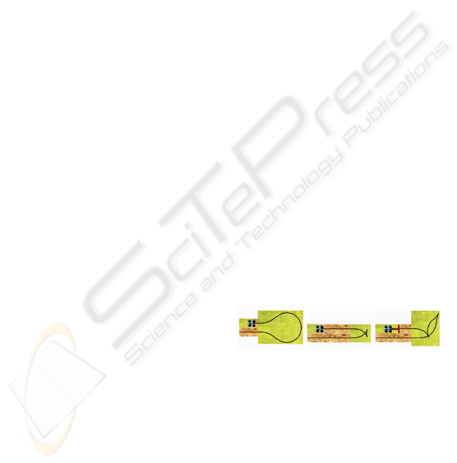
(a) Loop turn. (b) Fish-tail. (c) With trailer.
Figure 1: Different types of maneuver in headland.
Another solution is to perform reverse turns, i.e.
maneuvers executed with stop points and a reverse
motion as depicted in figures 1(b) and 1(c), leading
to reduced headlands. However, although more in
accordance with European agricultural practices, au-
tomation of such maneuvers in headland has rarely
been considered in the literature. In fact, numerous
approaches devoted to road applications have been
proposed for the autonomous maneuvers of a vehi-
cle, even with one or several trailers, see (Altafini C.,
2001), (Lamiraux F., 1998), (Hermosillo J., 2003),
109
Cariou C., Lenain R., Berducat M. and Thuilot B. (2010).
AUTONOMOUS MANEUVERS OF A FARM VEHICLE WITH A TRAILED IMPLEMENT IN HEADLAND.
In Proceedings of the 7th International Conference on Informatics in Control, Automation and Robotics, pages 109-114
DOI: 10.5220/0002875501090114
Copyright
c
 SciTePress

but most of these control algorithms seem not well-
adapted for an agricultural context. This paper pro-
poses to address the automation of the maneuvers of
a vehicle-trailer system, dedicated to an off-road con-
text. This paper extends our previous work (Car-
iou et al., 2009) where accurate fish-tail maneuvers
without trailer were autonomously performed. The
general 1-trailer system is here considered, i.e. the
trailer is hitched up at some distance from the middle
point of the rear axle of the vehicle.
2 MOTION PLANNER
With regard to the path planning problem of agri-
cultural machines in headland, generic optimal con-
trol algorithms are often investigated to find opti-
mal point-to-point trajectories for a given cost func-
tion from a wide variety of configurations, see (Vou-
gioukas et al., 2006). Primitive-based planning ap-
proaches are also widely used in the literature, re-
lying either on clothoids, polynomial splines or cu-
bic spirals to construct non-holonomic motions, see
(Lau B., 2009). We have studied a similar approach
well-adapted to agricultural maneuvers. It allows to
rapidly obtain an efficient path planning solution for
reverse turns of a vehicle-trailer system, based on ele-
mentary primitives (line segment, arc of circle) con-
nected together with pieces of clothoid in order to en-
sure curvature continuity.
2.1 Arc of Clothoid
The curvature c of a clothoid varies linearly with res-
pect to its curvilinear abscissa s (c = g.s), see figure 2.
An arc of clothoid BP
1
admissible for the considered
vehicle can then be defined in order to connect a line
segment AB to a circle of radius R. To avoid the sa-
turation of the steering actuator, R is chosen slightly
upper than the minimum curvature radius of the ve-
hicle. The proportionality coefficient g is computed
according to the maximum vehicle front-wheel an-
gular velocity (ω
a
= 20
◦
/s) and of the vehicle linear
velocity (v
ref
= 1.75m/s) during the reverse turn, see
(Cariou et al., 2009) for more details. In that way,
continuous curvature trajectories admissible for the
vehicle can easily be constructed.
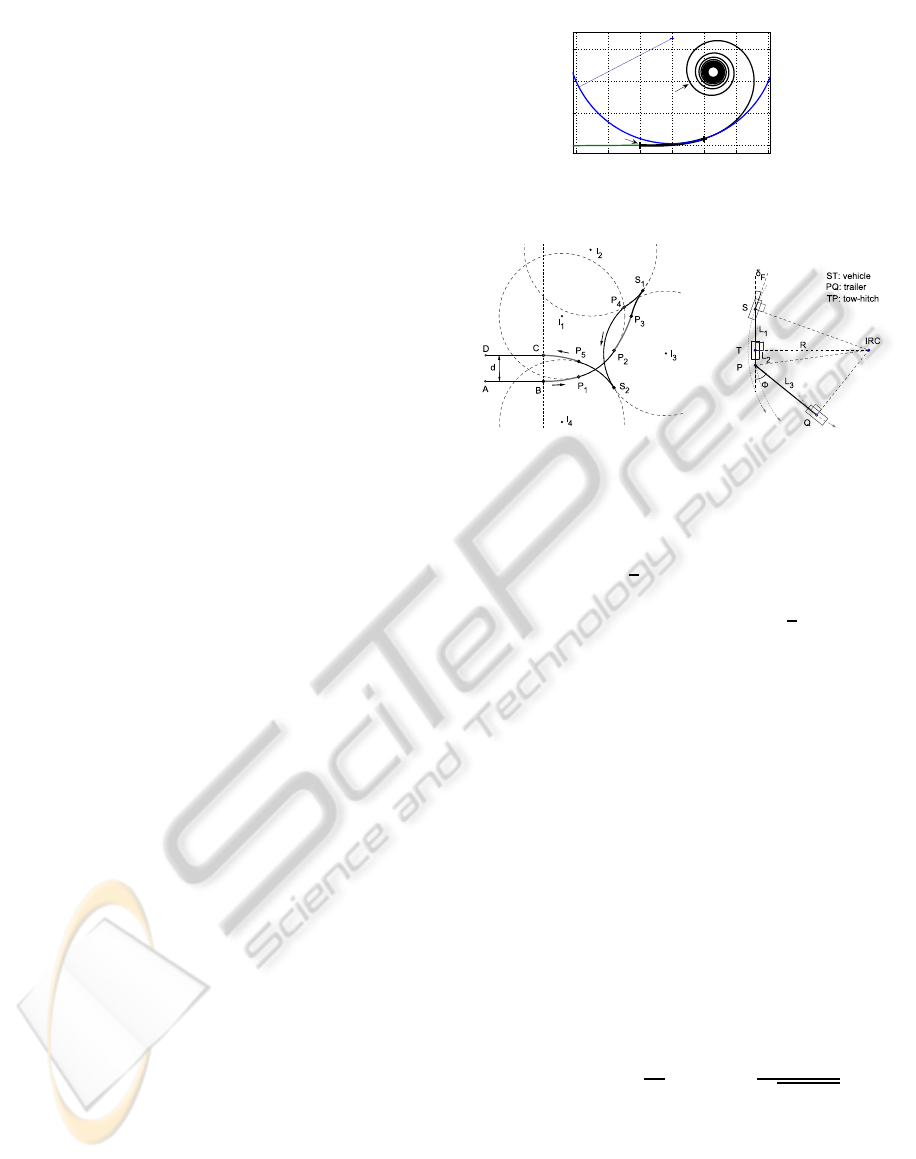
2.2 Trajectory Generation Strategy
The aim is to connect two adjacent tracks AB and CD
separated from a distance d, see figure 3(a). The pro-
posed strategy considers the following motions.
−2 −1 0 1 2 3 4
0
1
2
3
x(m)
y(m)
P
A
B
R
1
Clothoid
Figure 2: Clothoid, g = 0.15.
(a) Trajectories. (b) Rotation centers.
Figure 3: Path planning.
• The first movement from B to S
1
is composed of
an arc of clothoid BP
1
, to increase the curvature
from c = 0 to c =
1
R
, an arc of circle P
1
P
2
of center
I
1
and of radius R, a second arc of clothoid P
2
P
3
to decrease the curvature from c =
1
R
to c = 0,
and a part of a third arc of clothoid P
3
S
1
required
to align the trailer with the vehicle at the end of
the movement. Aligning the vehicle-trailer sys-
tem at the first stop point S
1
leads to a suitable
configuration to plan the reverse motion. At S
1
,
the wheels are reorientated to change the vehicle
instantaneous rotation center to I
2
.
• The reverse movement is then built, composed
firstly of an arc of circle S
1
P
4
to increase the
vehicle-trailer angle φ, see the notation in the bi-
cycle representation figure 3(b). The point P
4
is
determined in order that the vehicle-trailer system
reaches the configurationshown in figure 3(b): the
center of rotation of the trailer coincides with the
center of rotation of the vehicle, when the vehicle
front steering angle is set to a value δ
d
F
= 20
◦
. Ge-
ometrical considerations show that the expected
value φ
ref
for the angle φ is:
φ
ref
= π− arctan(
R
L
2
) −arccos(
L
3
q
R
2
+ L
2
2
) (1)
with: R = L
1
/tanδ
d
F
This is a stable configuration enabling a circular
motion of radius R when pure rolling without sli-
ding conditions are satisfied. It serves here as an
objective configuration. At P
4
, the wheels are re-
orientated to change the vehicle instantaneous ro-
ICINCO 2010 - 7th International Conference on Informatics in Control, Automation and Robotics
110

tation center from I
2
to I
3
. Then, an arc of circle
P
4
S
2
of center I
3
and radius R is built.
• The third movement is composed of an arc of cir-
cle S
2
P
5
of center I
4
and radius R, and an arc of
clothoid P
5
C to decrease the curvature from c =
1
R
to c = 0. S
2
is the second stop point, defined as the
intersection between the circles of center I
3
and I
4
.
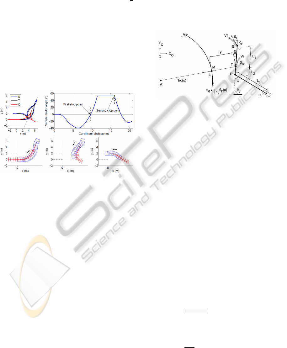
Figure 4 presents simulation results with two ad-
jacent tracks separated from a distance d = 2m. At the
first stop point S
1
, the vehicle-trailer angle is φ = 0
◦
,
i.e. the trailer and the vehicle are aligned, see the tra-
jectories of points S, T and Q, respectively the centers
of the vehicle front and rear axle and the center of the
trailer axle. During the reverse motion, the vehicle-
trailer angle reaches and maintains the expected con-
figuration φ
ref
(here φ
ref
= 53
◦
).
Figure 4: Path planning results.
3 CONTROL ALGORITHMS
3.1 Forward Motion
Accurate automatic guidance of mobile robots in
an agricultural environment constitutes a challenging
problem, mainly due to the low grip conditions usu-
ally met in such a context. In fact, as pointed out
in (Wang D., 2006), if the control algorithms are de-
signed from pure rolling without sliding assumptions,
the accuracy of path tracking may be seriously da-
maged, especially in curves. Therefore, sliding has
to be accounted in the control design to preserve the
accuracy of path tracking, whatever the path to be fol-
lowed and soil conditions.
3.1.1 Kinematic Model extended with Sliding
Parameters
In the same way than in (Lenain et al., 2006a), two
parameters homogeneouswith sideslip angles in a dy-
namic model, are introduced to extend the classical
kinematic model, see the bicycle representation of the
vehicle in figure 5. These two angles, denoted β
F
and
β
R
for the front and rear axle, represent the difference
between the theoretical direction of the linear velocity
vector at wheel centers, described by the wheel plane,
and their actual direction. These angles are assumed
to be entirely representative of sliding influence on
vehicle dynamics. The notations used in this paper
are listed below and depicted in figure 5.
Figure 5: Path tracking parameters.
• S and T are the centers of the front and rear virtual
wheel. T is the point to be controlled.
• θ
v
is the orientation of vehicle centerline with res-
pect to an absolute frame [O,X
O
,Y
O
).
• δ
F
is the front steering angle and constitutes the
first control variable.
• V
r
is the vehicle linear velocity at point T and
constitutes the second control variable.
• β
F
and β
R
are the front and rear sideslip angles.
• M is the point on the reference path Γ to be fol-
lowed, which is the closest to T.
• s is the curvilinear abscissa of point M along Γ.
• c(s) is the curvature of the path Γ at point M.
• θ
Γ
(s) is the orientation of the tangent to Γ at point
M with respect to the absolute frame [O,X
O
,Y
O
).
•
˜
θ = θ
v
− θ
Γ
is the vehicle angular deviation.
• y is the vehicle lateral deviation at point T.
• φ is the vehicle-trailer angle.
• L
1
= 1.2m and L
3
= 2.34m are respectively the
vehicle and trailer wheelbases. L
2
= 0.46m is the
vehicle tow-hitch.
The equations of motion are derived with respect
to the path Γ. It can be established, see (Lenain et al.,
2006a), that:















˙s = V
r
cos(
˜
θ−β
R
)
1−c(s) y
˙y = V
r
sin(
˜
θ− β
R
)
˙
˜
θ = V
r
[cos(β
R
)λ
1
− λ
2
]
˙
φ = −
V
r
L
1
L
3
[tanδ
F
(L
2
cosφ + L
3
) + L
1
sinφ]
(2)
AUTONOMOUS MANEUVERS OF A FARM VEHICLE WITH A TRAILED IMPLEMENT IN HEADLAND
111

with: λ
1
=
tan(δ
F
−β
F
)+tan(β
R
)
L
1
, λ
2
=
c(s)cos(
˜
θ−β
R
)
1−c(s) y
Model (2) accurately describes the vehicle motion
in presence of sliding as soon as the two additional pa-
rameters β
F
and β
R
are known. An observation algo-
rithm has been developed to achieve indirect estima-
tion, relying on the sole lateral and angular deviation
measurements, see (Lenain et al., 2006b).
3.1.2 Control Law Design
The extended model (2) constitutes a relevant basis
for mobile robot control design. As the vehicle-trailer
system is well-known for being naturally exponen-
tially stable when driving forward, the trailer is igno-
red in this case. In (Lenain et al., 2006a), the first
three equations in model (2) have been converted in
an exact way into linear equations, according to the
state and control transformations:
[s,y,
˜
θ] → [a
1
,a
2
,a
3
] = [s,y,(1− c(s)y) tan(
˜
θ+ β
R
)]
[V
r
,δ
F
] → [m
1
,m
2
] = [
V
r
cos(
˜
θ+β
R
)
1−c(s) y
,
da
3
dt
]
(3)
Finally, if derivativesare expressed with respect to
the curvilinear abscissa, the following chained form is
obtained:



a
′
2
=
da
2
da
1
= a
3
a
′
3
=
da
3
da
1
= m
3
=
m
2
m
1
(4)
Since chained form (4) is linear, a natural expres-
sion for the virtual control law m
3
is:
m
3
= −K
d
a
3
− K
p
a
2
(K
p
,K
d
) ∈ ℜ
+2
(5)
since it leads to:
a
′′
2
+ K
d
a
′
2
+ K
p
a
2
= 0 (6)
which implies that both a
2
and a
3
converge to zero,
i.e. y → 0 and
˜
θ → β
R
. The inversion of control trans-
formations provides the front steering control law:
δ
F
= β
F
+ arctan
n
− tan(β
R
)
+
L
1
cos(β
R
)
(
c(s)cos
˜
θ
2
α
+
Acos
3
˜
θ
2
α
2
)
o
(7)
with:



˜
θ
2
=
˜
θ− β
R
α = 1− c(s)y
A = −K
p
y− K
d
αtan
˜
θ
2
+ c(s)αtan
2
˜
θ
2
In addition, as the actuation delays and vehicle
inertia may lead to significant overshoots, especially
at each beginning/end of curves, a predictive action
must be added to the steering control in order to main-
tain accurate path tracking performances, see (Lenain
et al., 2006b) for more details. A second control loop
can be designed, dedicated to speed control. In (Car-
iou et al., 2009), a Model Predictive Control tech-
nique is used to anticipate speed variations and reject
signifiant overshoots in longitudinal motion.
3.2 Backward Motion
It is well-known that steering backward a vehicle-
trailer system has a tendency to jackknife, and re-
quires special driving skill. In the literature, nume-
rous path following approaches have addressed this
problem when the trailer is hooked directly at the cen-
ter of the rear axle of the vehicle. In contrast, the case
of deported trailers has been rarely considered. In this
paper, we propose to indirectly control the vehicle-
trailer angle. Two control strategies are proposed.
3.2.1 Regulation of the Vehicle-trailer Angle
With the motion planner described in subsection 2.2,
the previous steering control law (7) can be used du-
ring the backward motion until the vehicle-trailer sys-
tem presents the expected angle φ
ref
, corresponding
to the configuration at point P
4
depicted in figure 3(b).
Next, as the rest of the backward movement is quite
short to reach the stop point S
2
, the vehicle-trailer an-
gle can be simply stabilized on φ
ref
. More precisely,
relying on the fourth equation in model (2), the error
dynamic
˙
φ = K
R
(φ
ref
− φ) (K
R
> 0) can be imposed
with the following front-wheel steering control law:
δ
F
= arctan
−L
1
sinφ −
K
R
L
1
L
3
(φ
ref
−φ)
V
r
L
2
cosφ + L
3
(8)
3.2.2 Stabilization of the Trailer on the Planned
Trajectory
Another solution is to control the center of the trailer
axle on its respective planned trajectory, see the tra-
jectory of Q during the backward motion in figure 4.
For that, the trailer is first considered as an indepen-
dent virtual vehicle, with a rear steering wheel located
at the hitch point P and a fixed front-wheel located at
point Q, see figure 6. The control objective can then
be expressed as ensuring the convergence of this vir-
tual vehicle (moving forward) to the reference path
Γ. The first three equations in model (2) describe the
motion of such a vehicle, except that δ
F
has to be rem-
placed by −δ
c
, since the variations in the orientation
of the vehicle are inverted when rear steering is con-
sidering instead of front steering. The state variables
are now y
t
and
˜
θ = θ
t
− θ
Γ
, respectively the trailer
lateral and angular deviation, see figure 6. A chained
form transformation similar to the one presented in
ICINCO 2010 - 7th International Conference on Informatics in Control, Automation and Robotics
112

subsection 3.1 can then be applied, and the expected
value for δ
c
can be directly inferred from (7):
δ
c
= − arctan
n
L
3
(
c(s)cos
˜
θ
α
t
+
A
t
cos
3
˜
θ
α
2
t
)
o
(9)
with:

α
t
= 1 − c(s)y
t
A
t
= −K
p
y
t
− K
d
α
t
tan
˜
θ+ c(s)α
t
tan
2
˜
θ
δ
c
describes the desired direction of the linear ve-
locity ~v at the hitch point. Then, the vehicle-trailer
angle φ
ref
ensuring that the center of rotation of the
trailer coincides with the center of rotation of the ve-
hicle can easily be inferred from δ
c
via basic geomet-
rical relations, see figure 6:
φ
ref
= δ
c
+ arcsin
L
2
sinδ
c
L
3
(10)
Finally, the proposed angle φ
ref
can be controlled
just as in subsection 3.2.1: reporting (10) into (8) pro-
vides the front steering control law for the vehicle.
Figure 6: Trailer as a virtual vehicle.
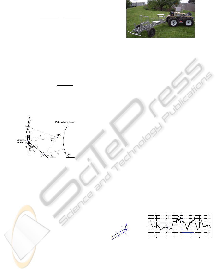
4 EXPERIMENTAL RESULTS
In this section, the capabilities of the proposed con-
trol algorithms are investigated on an irregular natu-
ral terrain, using the experimental vehicle-trailer sys-
tem depicted in figure 7. The vehicle is an all-terrain
mobile robot whose weight is 650kg. The only exte-
roceptive sensor is an RTK-GPS receiver, whose an-
tenna has been located straight up the center of the
vehicle rear axle. It supplies an absolute position ac-
curate to within 2cm, at a 10Hz sampling frequency.
The vehicle-trailer angle is measured using a poten-
tiometer. A gyrometer has also been added to obtain
an accurate heading of the vehicle during the maneu-
vers.
In the forthcoming experimental test, the objec-
tive for the vehicle-trailer system is to follow au-
tonomously two straight lines AB and CD sepa-
rated from 2m, see figure 8(a), and to execute au-
tonomously the reverse turn using control law (8).
The lateral deviation recorded at the center T of the
rear wheels, according to the curvilinear abscissa, is
Figure 7: Experimental vehicle-trailer system.
reported in figure 8(b). At the beginning, the vehi-
cle starts at about 25cm from the path to be followed.
Then, it reaches the planned path and maintains an
overall lateral error about ±15cm during the maneu-
ver. The main overshoots in the lateral deviation take
place at the moment of a large deceleration and accel-
eration on a sliding ground (curvilinear abscissas 15m
and 32m). Despite such conditions, the lateral devia-
tion remains inside ±15cm. This highlights the ca-
pabilities of the proposed algorithms, taking into ac-
count for sliding effects and actuator delays.
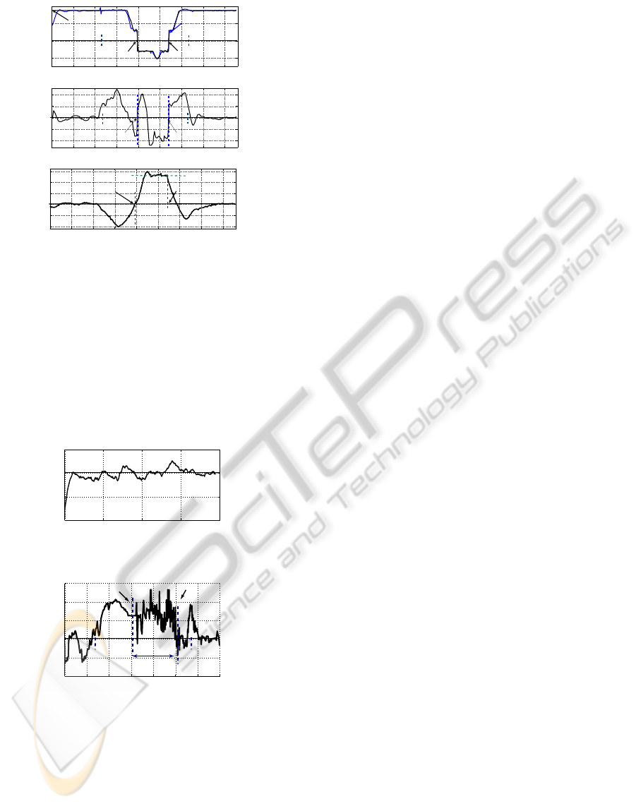
The vehicle speed is reported at the top of figure 9.
The speed reference v
ref
= 1.75m/s is correctly fol-
lowed, and the speed variations are satisfactorily an-
ticipated with the predictive approach. At the center
of figure 9 is reported the vehicle front steering angle.
It can be observed that its variations are quite smooth
and that the wheels are satisfactorily reorientated to
change the vehicle instantaneous rotation center at the
stop points as well as at point P
4
(curvilinear abscissa
22m). The vehicle-trailer angle w.r.t. the curvilinear
abscissa is reported at the bottom of figure 9. In accor-
dance with the simulations depicted in figure 4, this
angle reaches −40
◦
during the first movement. The
trailer and the vehicle are then aligned at the first stop
point. During the reverse motion, this angle increases
up to φ
ref
= 53
◦
(since here δ
d
F
= 20
◦
). The angle is
then correctly regulated to the value φ
ref
= 53
◦
.
A
B
C
D
(a) Paths.
0 5 10 15 20 25 30 35
−0.2
−0.15
−0.1
−0.05
0
0.05
0.1
0.15
0.2
Curvilinear abscissa(m)
Lateral deviation(m)
Fisrt stop point
Second stop point
Reverse
motion
B
C
(b) Lateral deviation at T (veh. rear axle).
Figure 8: Experimental results.
In the following test, the objective consists to val-
idate the control law proposed in subsection 3.2.2
for the stabilization of the vehicle-trailer system on
a planned trajectory. To this aim, a 80m-long ref-
erence path was first recorded during a preliminary
run achieved in manual driving with the mobile robot
moving forward. Then, the path is autonomously
AUTONOMOUS MANEUVERS OF A FARM VEHICLE WITH A TRAILED IMPLEMENT IN HEADLAND
113

0 5 10 15 20 25 30 35 40
−1
0
1
2
Curvilinear abscissa (m)
Speed (m/s)
Speed reference
Measured speed
First stop point
Second stop point
B C
0 5 10 15 20 25 30 35 40
−20
−10
0
10
20
Curvilinear abscissa (m)
Front steering angle (°/s)
First stop point Second stop point
B
C
0 5 10 15 20 25 30 35 40
−40
−20
0
20
40
60
Curvilinear abscissa (m)
Vehicle−trailer angle (°)
First stop point
Second stop point
Figure 9: Speed, front steering angle, and φ.
followed backward at 0.5m/s with the vehicle-trailer
system. At the beginning, the trailer starts with a lat-
eral deviation of 1m from the path to be followed.
Then, it reaches the planned path and maintains a sat-
isfactory overall lateral error about ±20cm. Finally,
the reverse turn maneuver depicted in figure 8(a) is
performed with this control law. The lateral deviation,
reported in figure 11, maintains an overalllateral error
within ±20cm during the maneuver.
0 20 40 60 80
−1
−0.5
0
0.5
Lateral deviation (m)
Curvilinear abscissa (m)
Figure 10: Reversing a vehicle-trailer system.
0 5 10 15 20 25 30 35
−0.2
−0.1
0
0.1
0.2
0.3
Curvilinear abscissa (m)
Lateral deviation (m)
Reverse motion
First stop point
Second stop point
B
C
Figure 11: Lateral deviation at Q (trailer axle).
5 CONCLUSIONS
This paper addresses the problem of path generation
and motion control for the autonomous maneuvers
of a farm vehicle with a trailed implement in head-
land. A reverse turn planner has been first presented,
based on primitives connected together with pieces
of clothoid, in order to ensure curvature continuity.
Next, control algorithms have been considered. When
the system is driving forward, the control algorithms
are based on a kinematic model extended with ad-
ditional sliding parameters and on model predictive
control approaches. When the system is driving back-
ward, two different steering controllers have been pre-
sented. Promising results are reported with an off-
road mobile robot pulling a trailer during reverse turn
maneuvers. In spite of a fast speed and high steering
variations, an overall tracking error within ±20cm is
obtained during the maneuver.
REFERENCES
Altafini C., Speranzon A., W. B. (2001). A feedback con-
trol scheme for reversing a truck and trailer vehicle.
In IEEE Transactions on robotics and automation,
17(6):915-922.
Cariou, C., Lenain, R., Thuilot, B., and Martinet, P. (2009).
Motion planner and lateral-longitudinal controllers for
autonomous maneuvers of a farm vehicle in headland.
In IEEE Intelligent Robots and Systems, St Louis,
USA.
Hermosillo J., S. S. (2003). Feedback control of a bi-
steerable car using flatness: application to trajectory
tracking. In IEEE Int. American Control Conference,
Denver, Co, USA, 4:3567-3572.
Lamiraux F., L. J. (1998). A practical approach to feedback
control for a mobile robot with trailer. In IEEE Int.
conf. on Robotics and Automation, Louvain, Belgique.
Lau B., Sprunk C., B. W. (2009). Kinodynamic motion
planning for mobile robots using splines. In IEEE In-
telligent Robots and Systems, St Louis, USA.
Lenain, R., Thuilot, B., Cariou, C., and Martinet, P. (2006a).
High accuracy path tracking for vehicles in pres-
ence of sliding: Application to farm vehicle auto-
matic guidance for agricultural tasks. In Autonomous
Robots, 21(1):79-97.
Lenain, R., Thuilot, B., Cariou, C., and Martinet, P.
(2006b). Sideslip angles observer for vehicle guid-
ance in sliding conditions: application to agricultural
path tracking tasks. In IEEE Int. conf. on Robotics and
Automation, Orlando, USA.
Vougioukas, S., Blackmore, S., Nielsen, J., and Fountas, S.
(2006). A two-stage optimal motion planner for au-
tonomous agricultural vehicles. In Precision Agricul-
ture, 7:361-377.
Wang D., L. C. B. (2006). Modeling skidding and slipping
in wheeled mobile robots: control design perspective.
In IEEE int. conf. on Intelligent Robots and Systems,
Beijing, China.
ICINCO 2010 - 7th International Conference on Informatics in Control, Automation and Robotics
114