OBSTACLES AVOIDANCE IN THE FRAME WORK
OF PYTHAGOREAN HODOGRAPH BASED PATH PLANNING
M. A. Shah
*
, A. Tsourdos, P. M. G. Silson, D. James and N. Aouf
Dept. of Informatics and Sensors, Cranfield University, Cranfield, U.K.
Keywords: Pythagorean Hodograph, Bending energy, Path Planning, Feasible paths.
Abstract: This paper deals with the problem of obstacle avoidance in the path planning based on Pythagorean
Hodograph. The proposed obstacle avoidance approach is based on changing the curvature in case of
Pythagorean Hodograph curves. However this may result in an increase in the length of the path.
Furthermore in some cases obstacle avoidance by changing the curvature of the path may result not only in
an increase in path length but also to a tremendous increase in bending energy. An increase in bending
energy of a path as a result of curvature change above certain limit makes the path very difficult or
impossible to fly.
1 INTRODUCTION
In path planning for UAVs the obstacle avoidance is
a common problem. In literature different researcher
adopted different ways to solve the problem of
obstacle avoidance depending on the context of the
problem. (Madhavan at el 2006) and (H. Bruyninckx
at el 1997) proposed a solution to avoid the obstacle
in case of the Pythagorean Hodograph based path
planning for UAVs by manipulating the curvature of
the PH path. By changing the curvature of the path
an obstacle can be avoided but the path length is
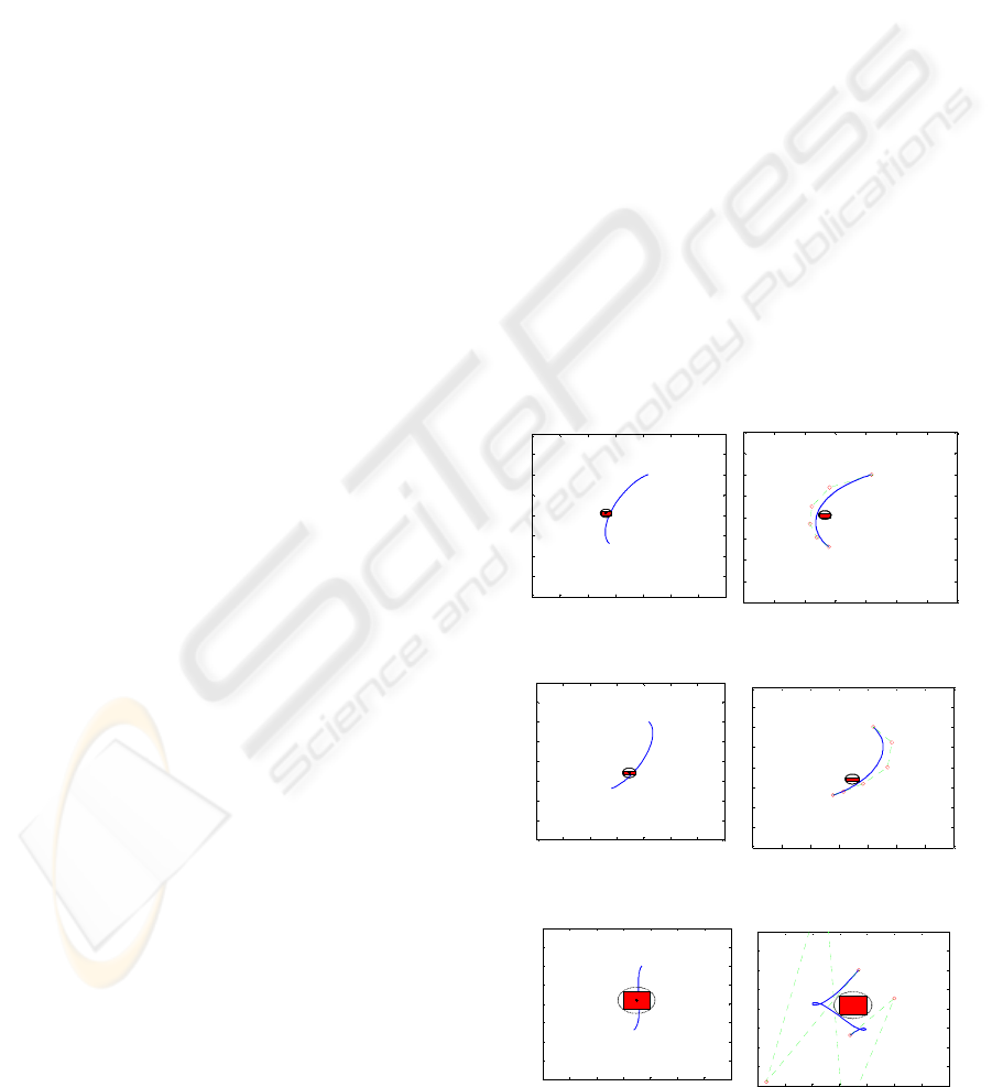
increased tremendously as a result. For example
figure 1and 2 illustrate this fact:
But sometimes situations arise where obstacles
avoidance by changing the curvature of the path
results in path of very high bending energy. A path
with a very high bending energy is very difficult for
UAVs to follow and hence not a feasible path.
Figure 3 shows this fact.
Therefore curvature manipulation method can
not be solely used for obstacle avoidance in PH
based path planning because it is bound to fail for
some cases. We need an alternative method for
obstacle avoidance which can guarantee feasible
(safe and flyable) paths. To elaborate such a method
is the subject of this paper.
The rest of the paper is organized as follows:
Section 2 describes the problem formulation. Section
3 introduces the Pythagorean Hodograph to generate
the initial paths. Section 4 introduces the proposed
solution to the problem. Section 5 discusses the
simulation results and finally section 6 draws the
conclusion.
-20 -10 0 10 20 30 40 50
-20
-10
0
10
20
30
40
50
60
Path with Obstacles
X co m
p
onent of the curve meters
Y component of the curve meters
-20 -10 0 10 20 30 40 50
-20
-10
0
10
20
30
40
50
60
2D Quintic Bezier Curve
Figure 1: Obstacle avoidance by curvature change.
-20 -10 0 10 20 30 40 50
-20
-10
0
10
20
30
40
50
60
Path with Obstacles
X component of the curve meters
Y component of the curve meters
-20 -10 0 10 20 30 40 50
-20
-10
0
10
20
30
40
50
60
2D Quintic Bezier Curve
Figure 2: Obstacle avoidance by curvature change.
-20 -10 0 10 20 30 40 50
-20
-10
0
10
20
30
40
50
60
Path with Obstacles
X co m
p
onent of the curve meters
Y component of the curve meters
-20 -10 0 10 20 30 40 5
0
-20
-10
0
10
20
30
40
50
60
2D
Q
uintic Bezier
C
urve
Figure 3: Obstacle avoidance by curvature change.
335
Shah M., Tsourdos A., M. G. Silson P., James D. and Aouf N. (2010).
OBSTACLES AVOIDANCE IN THE FRAME WORK OF PYTHAGOREAN HODOGRAPH BASED PATH PLANNING..
In Proceedings of the 7th International Conference on Informatics in Control, Automation and Robotics, pages 335-339
DOI: 10.5220/0002877803350339
Copyright
c
 SciTePress

2 PROBLEM FORMULATION
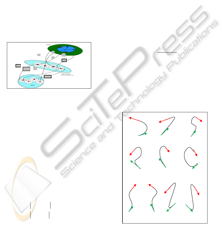
A mission is planned to fly a group of unmanned
aerial vehicles safely from base B to target T as
shown in Figure 4. All vehicles start from the base at
the same time. The environment contains stationary
and moving obstacles. During the flight, the vehicles
will avoid inter-collision and collision with the
stationary and moving obstacles. Initially, UAV
paths are planned offline by the path planning
module (Path Planner) on the basis of the available
knowledge about the environment. The UAVs start
following these paths, if during the flight any of the
UAVs comes across an obstacle, which was not
known before then changes are made to the initial
path of corresponding UAV to avoid the obstacles
while maintaining UAVs cooperation.
Figure 4: Swarm of UAVs Scenario.
The base and the goal points for each UAV are
specified by initial and final poses. Let the starting
pose of the i
th
UAV in the terms of its position and
orientation is
),,,(
sisisisisi
zyxP
θ
and the final
pose of the same UAV is
),,,(
fififififi
zyxP
θ
then
the path of the UAV is defined as a parametric curve
r(t) = [ x(t), y(t), z(t) ] such that the kinematics and
dynamic constraints of the vehicle are satisfied.
Mathematically this can be written as:
)(),,,,(
ssisisisisisi
trzyxP =
φ
θ
)(),,,,(
ffifififififi
trzyxP =
φ
θ
),,,,(),,,,(
)(
fifififififi
tri
sisisisisisi
zyxPzyxP
i
φθφθ ⎯⎯→⎯
Subjected to:
max
max
)(
)(
ττ
κκ
≤
≤
t
t
i
i
With curvature
i
k
and torsion
i
τ
for i=1,..,n , n
is the number of cooperating UAVs. In case of
obstacle interruption these initial paths are modified
such that the modified path is feasible (collision free
and flyable). We assume in the developments of our
paper that the UAVs are flying at a constant altitude.
How we generate these paths is explained in the next
section.
3 PROPOSED SOLUTION TO
THE PROBLEM
The initial trajectories of the UAVs are calculated
from known initial and final poses. Therefore the
poses play a pivotal rule in generating and
modifying these trajectories. For each path there are
two poses i.e the initial pose and final pose. The
orientation of these poses could be from any of the
four quadrants of Cartesian plane. Since there are
total of four quadrants, and any two quadrant can be
selected at a time for two orientation (one for initial
pose and one for final pose), therefore we can have a
total of:
4
4!
6
2
(4 2)! 2!
⎛⎞
=
=
⎜⎟
−×
⎝⎠
possible cases. These cases are shown in the figure 5
as a, b, c, d, e and f. There are four more possible
cases if the initial and final poses are taken from the
same quadrant. These cases are shown in figure 5 as
g, h, i and j. The orientations corresponding to initial
poses are represented by green arrow and the
orientations corresponding to the final poses are
represented by red arrow. Referring to the figure 5
below, we have the following cases:
a
b
c
d
e
f
g
h
i
j
Figure 5: All possible combinations of the initial and final
pose taken from four quadrant.
Case a: The initial pose belongs to quadrant 1 and
the final pose belongs to quadrant 2. i.e.
ICINCO 2010 - 7th International Conference on Informatics in Control, Automation and Robotics
336

0
2
si
π
θ ≤≤
and
2
fi
π
θ
π ≤≤
Case b: The initial pose belongs to quadrant 1 and
the final pose belongs to quadrant 3:
0
2
si
π
θ ≤≤
and
3
2
fi
π
πθ ≤≤
Case c: The initial pose belongs to quadrant 1 and
the final pose belongs to quadrant 4:
0
2
si
π
θ ≤≤
and
32
2
fi
π
θ
π ≤≤
Case d: The initial pose belongs to quadrant 2 and
the final pose belongs to quadrant 3:
2
si
π
θ
π ≤≤
and
3
2
fi
π
πθ ≤≤
Case e: The initial pose belongs to quadrant 2 and
the final pose belongs to quadrant 4:
2
si
π
θ
π ≤≤
and
32
2
fi
π
θ
π ≤≤
Case f: The initial pose belongs to quadrant 3 and
the final pose belongs to quadrant 4:
3
2
si
π
πθ ≤≤
and
3
2
fi
π
θ
π ≤≤
Case g: both the initial pose and the final pose
belong to quadrant 1:
0,
2
si fi
π
θθ ≤≤
Case h: both the initial pose and the final pose
belong to quadrant 2:
,
2
si fi
π
θ
θπ ≤≤
Case i: both the initial pose and the final pose belong
to quadrant 3:
,3
2
si fi
π
πθθ ≤≤
Case j: both the initial pose and the final pose belong
to quadrant 4:
3,2
2
si fi
π
θ
θπ ≤≤
Now cases a, b, e and f are safe as shown by figure 1
and figure 2 in the introduction section.
Cases c, d, g, h, i and j have the possibility to give
paths of unacceptably higher bending energy when
manipulated to avoid obstacles. Therefore they
needed some method such that safe and flyable paths
are produced.
The method to avoid the obstacle in the case of c,
d, g, h, i and j (unsafe cases) comprise of introducing
an intermediate waypoint (pose) somewhere
between the initial and final pose such that the first
and second pose, and, second and third pose can be
connected by two PH quintic curves. Each of these
two individual PH component becomes like one of
the case a, b, e or f.
Since pose is a combination of position and
direction, therefore the position and direction of the
inserted intermediate pose must be determined. The
following paragraphs describe the determination of
the position and direction.
4.1 Position of the Intermediate Pose
Referring to the figure 6, if (, )
cen cen
xy are the
coordinates of the centre of the obstacle,
d
r is the
radius of the circle enclosing the obstacle, then the
coordinates of the points of the circle enclosing the
obstacle are (x, y) given by the following equations:
cos
cen d
xx r
θ
=
+
sin
cen d
yy r
θ
=+
Where
[0 2 ]
θ
π
∈
The position
(, )
iwp iwp
xy corresponding to the new
waypoint is given by:
cos
iwp saf cn d
xdxr
ξ
=
++
 sin
iwp saf cn d
ydyr
ξ
=
++ 
2
π
ξ
=
, if the UAV is approaching from the bottom
of the obstacle.
ξ
π
=
, if the UAV is approaching from the right.
3
2
π
ξ =
,if the UAV is approaching from the top. 
0
ξ
=
,if the UAV is approaching from the left.
saf
d
is the safety distance.

Figure 6: Position specification of the intermediate
waypoint.
4.2 Direction of the Intermediate Pose
The intermediate waypoint is inserted between the
initial and final poses. The direction of the
intermediate waypoint
iwp
θ
is such that when the two
consecutive poses are connected via PH quintic in
case of c, d, g, h, i and j each individual PH segment
becomes like one of the cases a, b, d or e. We
consider each individual case separately.
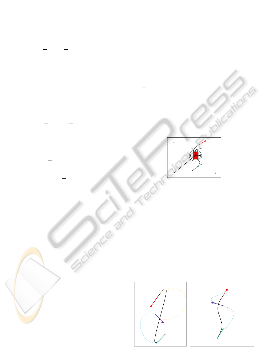
Case g, i: If both the directions of initial and final
poses belong to quadrant 1 or quadrant 3 then the



Initial pp
Final pose
Intermediate
pose
Alternative path
Figure 7: Direction of intermediate waypoint for cases g
and i.

Position

OBSTACLES AVOIDANCE IN THE FRAME WORK OF PYTHAGOREAN HODOGRAPH BASED PATH
PLANNING.
337

direction of intermediate pose is
2
iwp si
π
θθ =+
Case h, j: If both the directions of initial and final
poses belong to quadrant 2 or quadrant 4 then the
direction of intermediate pose is
2
iwp si
π
θθ =−
Case c: If the directions of initial pose belong to
quadrant 1 and that of final poses belong to quadrant
4 then the direction of intermediate pose is
2
iwp si
π
θθ =+
Case c inverted: If the directions of initial pose
belong to quadrant 4 and that of final poses belong
to quadrant 1 then the direction of intermediate pose
is
2
iwp si
π
θθ =−
This is shown in figure 9.






Figure 8: Direction of intermediate waypoint for cases h and j.





Figure 9: Direction of intermediate waypoint for cases c
and c inverted.
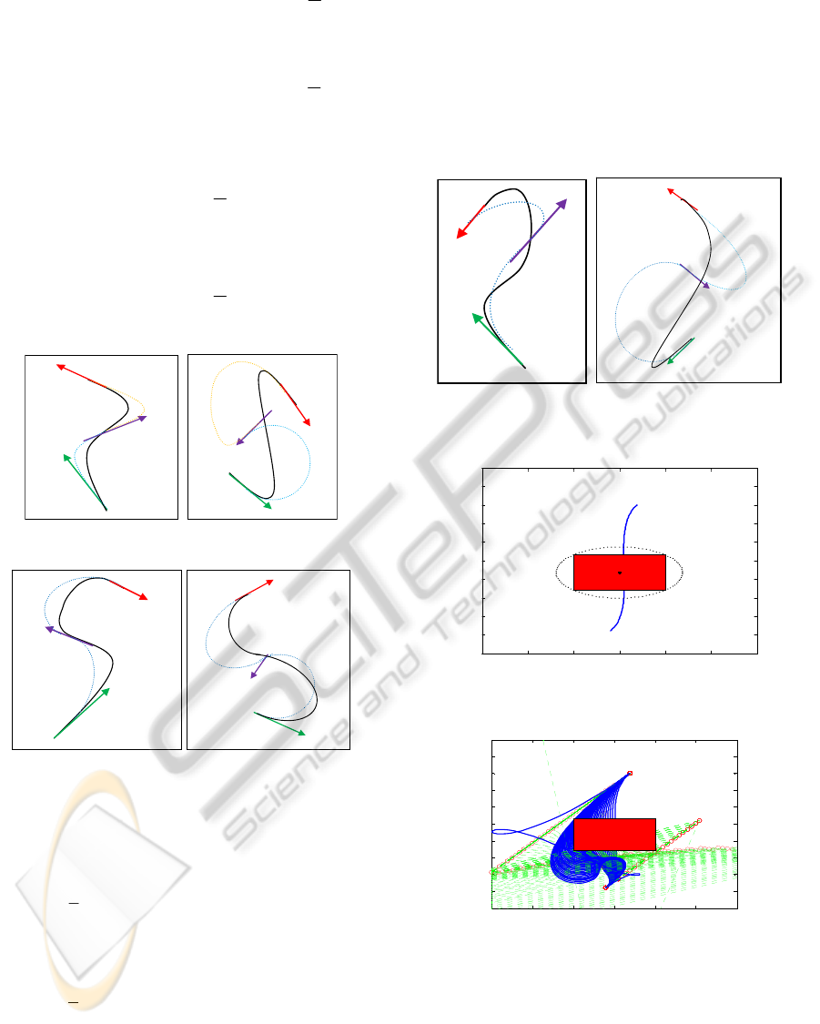
Case d: If the directions of initial pose belong to
quadrant 2 and that of final poses belong to quadrant
3 then the direction of intermediate pose
is:
2
iwp si
π
θθ =−
Case d inverted: If the directions of initial pose
belong to quadrant 3 and that of final poses belong
to quadrant 2 then the direction of intermediate pose
is
2
iwp si
π
θθ =+
4 SIMULATION RESULTS
The simulation results are obtained y taking only
one case in which the direction of initial and final
poses belong to quadrant 1. The method can be
tested for the rest of cases. The two methods (the
curvature manipulation method and the proposed
method) were simulated by taking the initial pose
(14, 6, 60
o
) and final pose (17, 40, 60
o
). The
following results were obtained.
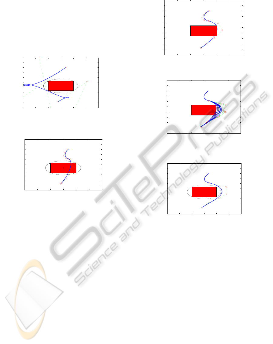
Figure 11 shows the path and the obstacle (red
rectangle).






Figure 10: Direction of intermediate waypoint for cases d
and d inverted.
0 5 10 15 20 25 30
0
5
10
15
20
25
30
35
40
45
50
Path with Obstacles
X component of the curve meters
Y component of the curve meters
Figure 11: The path with the obstacle.
0 5 10 15 20 25 30
0
5
10
15
20
25
30
35
40
45
50
Paths Avioding Obstacles
Figure 12: The path with different stages of curvature
manipulation to avoid the obstacle.
When the curvature manipulation method was
applied to avoid the obstacle (figure 12), the result
was a path with an unacceptable bending energy as
shown in the figure 13. The path shown in the figure
13 is not a flyable path because its high bending
energy makes it difficult to obey the dynamic
constraints. If we try to impose the dynamic
ICINCO 2010 - 7th International Conference on Informatics in Control, Automation and Robotics
338

constraints then its length will be increased
tremendously. The proposed method can offer a
remedy to this problem. The proposed method is
applied to insert an intermediate pose between the
initial and final pose. Then the three poses were
connected by the application of Pythagorean
Hodograph curves such that the individual curves
comply with the afore mentioned safe cases.
0 5 10 15 20 25 30
0
5
10
15
20
25
30
35
4
0
4
5
50
2D Quintic Bezier Curve
Figure 13: The final obstace free path with very high
bending energy.
0 5 10 15 20 25 30
0
5
10
15
20
25
30
35
40
45
50
X com
p
onent of the curve meters
Y component of the curve meters
Minimum Energy Curves
Figure 14: The path with same initial and final poses
resulted from the proposed method.
The result is shown in the figure 14. Figure 15 show
the same path after imposing the dynamic
constraints. Figure 16 shows the iterative process to
avoid the obstacle. Figure 17 shows the final
obstacle free path. The path shown in figure 17
obeys the dynamic constraints. The binding energy
is much lower compared to the path achieved with
the curvature manipulation method. The length of
the path is optimal as well.
5 CONCLUSIONS
The curvature manipulation method fails to give
feasible paths if the angle of the initial pose and final
pose in the first quadrant is increased above 60
o
and
55
o
on the upper side and decreased below 40
o
and
30 on the lower side. Therefore the operational angle
band of the method is very narrow which makes it
unsuitable for practical purposes. The proposed
method can accommodate poses with all the angles.
More over the path length of the resultant path is
optimal.
0 5 10 15 20 25 30
0
5
10
15
20
25
30
35
40
45
50
Curves with Curvature Constraints
Figure 15: The path with curvature constraint.
0 5 10 15 20 25 30
0
5
10
15
20
25
30
35
40
45
50
Paths Avioding Obstacles
Figure 16: The curvature manipulation of the path to avoid
the obstacle.
0 5 10 15 20 25 30
0
5
10
15
20
25
30
35
40
45
50
2D Quintic Bezier Curve
Figure 17: The obstacle free path with reasonable bending
energy and reasonable path length.
ACKNOWLEDGEMENTS
This research was sponsored by Engineering
Physical Science Research Council (EPSRC) and
British Aerospace (BAE Systems). Support is
gratefully acknowledged and appreciated by the
authors.
REFERENCES
S. Madhavan, A. Tsourdos, B. White. “A Solution to
Simultaneous Arrival of Multiple UAVs using
Pythagorean Hodograph” American Control
Conference, Minnesota USA, June 2006.
H. Bruyninckx, D. Reynaerts, “Path planning for mobile
and hyper redundant robots using Pythagorean
hodograph curves”, In 8
th
International Conference on
Advanced Robotics, ICAR, 97 pages 595-600, 1997.
OBSTACLES AVOIDANCE IN THE FRAME WORK OF PYTHAGOREAN HODOGRAPH BASED PATH
PLANNING.
339