
IDENTIFICATION OF DISCRETE EVENT SYSTEMS
Implementation Issues and Model Completeness
∗
Matthias Roth
1,2
, Lothar Litz
1
and Jean-Jacques Lesage
2
1
Institute of Automatic Control, University of Kaiserslautern, Germany
2
LURPA, Ecole Normal Sup
´
erieur de Cachan, France
Keywords:
Discrete event systems, Identification, Implementation.
Abstract:
This paper presents some practical issues for the identification of discrete event systems (DES). The considered
class of systems consists of a plant and a controller running is a closed-loop. Special emphasis is given
to a data collection procedure using industrial controllers and its impact on the external DES-behavior of
the considered systems. For models identified on the basis of observed external DES behavior using the
algorithm from (Klein, 2005) it is shown that under some conditions, the identified model language simulates
the complete original system language even if only a subset of this language is available for identification. This
model characteristic is crucial for many model-based techniques like diagnosis or verification. Analyzing the
observed data of a laboratory facility it is shown how it can be decided if the conditions for a complete model
hold for an existing application.
1 INTRODUCTION
Model-based techniques play a key role in many mod-
ern control applications. For systems that can be
modeled as Discrete Event Systems (DES) various
approaches to improve system dependability using
model-based methods have been proposed in the last
two decades. Examples for these methods are diag-
nosis (Sampath et al., 1996) and formal verification
with model checking (Machado et al., 2006). A bot-
tleneck for the application of model-based techniques
is the process of model-building which is usually ex-
pensive due to high costs for the necessary specialists.
A promising way to facilitate the use of model-based
methods is to offer efficient identification methods in
order to decrease the cost of model-building.
First approaches for the identification of DES have
been proposed in the sixties and seventies of the last
century in the field of computer science (Biermann
and Feldman, 1972). The identification of physical
systems which is a typical interest in many engineer-
ing domains is not the aim of these works. More re-
cent works especially on identification of Petri nets
are summarized in (Fanti and Seatzu, 2008). In
the last years two main directions of constructing a
∗
This works was partially supported by a grant from
R
´
egion
ˆ
Ile-de-France
Petri net from samples of its language have been fol-
lowed: In the first class of approaches specific rules
about interdependencies of observed events are used
to identify a Petri net on the basis of observed firing
and marking sequences (Meda-Campana and Lopez-
Mellado, 2005). The second class of approaches uses
optimization techniques like integer programming to
derive a Petri net structure according to given con-
straints (Giua and Seatzu, 2005), (Dotoli et al., 2006).
The main obstacle for the application of these
methods to real world systems is their relatively high
degree of abstraction. The work is usually not focused
on questions like how to represent data that can be
captured from a real system and how to cope with
inadequacies inherent to the data collection process.
In (Dotoli et al., 2006) a case study shows that there
is a considerable potential of identification methods
to obtain meaningful DES models of physical sys-
tems. Since the identification data base in this work
has been obtained by simulating a three tank system,
important issues of working with data captured from
a real system have not been addressed.
In (Klein et al., 2005) an algorithm for the iden-
tification of closed-loop DES is presented. The algo-
rithm has been designed to work with data obtained
from real systems and yields a monolithic automaton.
In this paper some implementation issues concerning
the application of this algorithm to a real system are
73
Roth M., Litz L. and Lesage J. (2010).
IDENTIFICATION OF DISCRETE EVENT SYSTEMS - Implementation Issues and Model Completeness.
In Proceedings of the 7th International Conference on Informatics in Control, Automation and Robotics, pages 73-80
DOI: 10.5220/0002879900730080
Copyright
c
SciTePress

presented. In section 2 the class of closed-loop DES
is presented and it is outlined that this system class
is an appropriate modeling formalism for many in-
dustrial systems. Section 3 summarizes some prac-
tical implications of the data collection procedure and
defines an appropriate data format for the identifica-
tion algorithm. The identification algorithm is com-
pactly presented in section 4. An important property
of models identified with this algorithm is proofed in
this section: Under some well-defined conditions con-
cerning the observed system language, the identified
model is able to simulate the complete original sys-
tem language of arbitrary length
1
. In section 5 the
data collection procedure and the identification algo-
rithm are applied to a laboratory facility in order to
show the relevance of the approach for real systems.
It is shown how it can be decided of if the precondi-
tions presented in the former section hold only using
measured system data.
2 CLOSED-LOOP DES
A typical configuration of industrial systems is a
closed-loop of controller and plant. In the plant, a
set of sensors measures certain process values and de-
livers them to the controller using the controller in-
puts. The controller executes a control algorithm and
determines appropriate actuator settings for the plant.
Commands to actuators in the plant are transfered via
controller output signals. Figure 1 shows this princi-
ple.
Figure 1: Closed-loop Discrete Event system.
The external behavior of such systems can be ob-
tained by an analysis of the signals exchanged be-
tween controller and plant. In the considered class
of systems these signals are binary. From an exter-
nal point of view, a signal changes its value asyn-
chronously which can be considered as the occurrence
of an event. The closed-loop system can be charac-
terized as non-deterministic since it consists of the
combination of a deterministic subsystem (controller)
and a non-deterministic subsystem (plant). Since the
closed-loop system does not have any inputs, it must
1
Language L
A
simulates language L
B
if L
A
⊇ L
B
holds
be considered as an event generator (note that the
controller inputs also belong to the external behav-
ior of the closed-loop DES). This system character-
istic shows that the application of test functions for
identification purposes like it is often done in contin-
uous systems is not possible for industrial closed-loop
DES. Only passive identification approaches work-
ing on observed system evolutions are suitable for the
considered system class.
The aim of identification is to deliver a model to
reproduce the external behavior of the closed-loop
system. Hence, it is necessary to capture the signals
exchanged between controller and plant in order to get
samples of the external system behavior. In case of
existing industrial facilities this process must be non-
invasive to avoid disturbances of the process. In the
next section, a method to capture these signals in an
efficient way is presented.
3 DATA COLLECTION
3.1 Technical Implementation
The implementation of a data collection procedure for
closed-loop DES necessitates capturing the signals
exchanged between plant and controller. The most ac-
curate approach to get the according signal values is
to connect the wires between sensors or actuators and
the controller with a special data collection hardware
like described in (de Smet et al., 2001). Although
such an approach is possible within a laboratory en-
vironment, for existing industrial facilities the neces-
sary cabling effort would be too important. Since one
of the main reasons to use identification methods is to
save costs, the effort to apply the method must not ex-
ceed the costs of manually model building. A slightly
less accurate data collection approach that can be im-
plemented with less effort is to collect the signals after
they have been captured by the controller.
Figure 2 shows the functional principle of a pro-
grammable logic controller (PLC) which is a widely
used class of controllers in industry. The controller
cyclically performs the steps ’input reading’ where it
reads the signals from the sensors, ’program execu-
tion’ to determine new output values for the actua-
tors, and ’output writing’ where the newly determined
commands are sent to the plant actuators. Modern
PLCs are equipped with a communication processor
which makes it possible to send the values of the in-
put and output signals to a standard PC where they can
be stored in a data base. The implementation of such
a connection is relatively easy (it is mainly a software
problem) and does not require any special hardware.
ICINCO 2010 - 7th International Conference on Informatics in Control, Automation and Robotics
74

Figure 2: PLC cycle and data collection.
As implementation of the data link between con-
troller and identification data base, a UDP (User Data-
gram Protocol) connection is used. At the end of the
’program execution’ phase, the communication pro-
cessor of the controller sends a UDP-datagram which
is received by the PC with the identification data
base. In order to validate that this connection is fast
enough to be used for data collection, tests have been
performed using a Siemens PLC (CPU 315-2 DP)
equipped with a program leading to a PLC-cycle time
of 25 to 30 ms. The PLC as a communication proces-
sor (CP 343-1 IT) which sends the data to a standard
PC (identification data base). Figure 3 shows that the
time between the reception of two packages alters be-
tween 25 ms and 30 ms according to the slightly vary-
ing PLC-cycle. It could also be observed that no data
packets got lost during the transmission. This shows
that the UDP connection is adapted for our purposes.
Figure 3: Validation of the UDP connection.
When the signal values are sent to the identifica-
tion data base, they are grouped in the controller I/O
(input/output) vector defined as follows:
Definition 1 (Controller I/O vector). Given r different
controller inputs I
1
, ..., I
r
and s different controller
outputs O
1
, ..., O
s
, the controller I/O vector u = (IO
1
,
..., IO
m
) with m = r + s is given by IO
i
= I
i
∀ i =
1,..,r and IO
r+1
= O
i
∀ i = 1,..,s. m = |u| denotes
the length of the vector (number of controller I/Os).
The controller I/O vectors which are sent to the
identification data base differ slightly from the real
values of the signals. Three scenarios are considered
to describe how the controller I/O vector captured in
the data base is affected by the data collection process
at the end of the ’program execution’ step in the PLC.
Figure 4 shows the evolution of two controller in-
puts (sensor values) in the plant. It can be seen that
the two signals change their values at different times
since the according sensors are not triggered simulta-
neously. In the middle of the figure, the PLC-cycle is
shown over time. The dotted line indicates that the
input values of the plant are read by the PLC dur-
ing the step ’input reading’. After the program exe-
cution phase, the input values are sent to the identifi-
cation data base. The evolution of the data received
in the data base (the sampled data) is shown below
the PLC cycle. Since the real values of the two inputs
have been captured simultaneously during the ’input
reading’ phase they also change their value simulta-
neously in the identification data base. As a conse-
quence for the identification algorithm it is important
to use an appropriate definition of the notion event.
Since in DES theory events cannot occur simultane-
ously it is not possible to define the change in value
of one signal as an event like it would probably be
the most intuitive way. Instead we use the following
definition:
Definition 2 (Event). The appearance of an event
leads to a new I/O vector u( j) with u( j) 6= u( j − 1).
Only I/O vectors generated by events are stored in the
data base.
As a consequence of the this definition, two suc-
cessive I/O vectors u( j) and u( j + 1) always differ in
at least one (but possibly more than one) I/O value.
In figure 5 a scenario with a controller input and
a controller output is shown. In the example it is
assumed that there is a logical condition in the con-
trol algorithm relating these two signals: if the input
changes its value, the controller changes the value of
the output as a consequence. It can be seen that the
cause (change in value of the input) and the accord-
ing effect (change in value of the output) are sent si-
multaneously to the data base. Hence, in the data
base cause and effect cannot not directly be seen. Ad-
ditionally, the figure shows that using the described
data collection procedure it is possible to receive I/O
vectors in the data base before the according output
values are valid for the plant. The output values are
sent to the plant during the step ’output writing’ which
takes place after the transfer of the I/O vector.
The third scenario in figure 6 shows the case of an
actuator influencing a sensor in the plant. When the
according output is set in the controller it is transfered
to the data base and with a short delay written to the
the plant. The actuator controlled by the output can
only then start influencing the sensor connected with
IDENTIFICATION OF DISCRETE EVENT SYSTEMS - Implementation Issues and Model Completeness
75

Figure 4: Sampling scenario 1.
Figure 5: Sampling scenario 2.
input 1. Hence, in this case cause and effect cannot
be captured simultaneously since the change in value
of input 1 occurs some time after the vector with the
change in value of output 1 has been sent to the iden-
tification data base. The delay of cause and effect is
often not considered in manually built models like in
(Sampath et al., 1996). A second issue of the data
collection process can also be seen in the figure: al-
though input 1 and output 1 change their value rela-
tively fast one after the other (faster than the duration
of a PLC-cycle), it can take up to one PLC cycle until
this change in value is sent to the identification data
base.
Figure 6: Sampling scenario 3.
The three scenarios show that the selected data
collection procedure introduces some inadequacies
that will also be part of the identified model. It is
thus important to clearly indicate when the data has
been captured in the PLC-cycle to precisely describe
the data in the identification data base.
3.2 Definition of the Observed
Language
For identification, the captured system data can be
interpreted as the language of the considered closed-
loop DES. The identification is based on the observa-
tion of I/O vector sequences during l
h
different system
evolutions:
Definition 3 (I/O vector sequence). If during the h-th
system evolution l
h
I/O vectors u
h
have been ob-
served, the sequence is denoted as σ(h) = (u
h
(1),
u
h
(2), . . . , u
h
(l
h
)).
The term ’system evolution’ refers to a system run
of a certain length. In manufacturing systems such an
evolution can be a production cycle. Based on the I/O
vector sequences it is possible to define the observed
word set (I/O vector sequences of a given length) and
the observed language:
Definition 4 (Observed word set and language).
The observed words of length q captured during p
different system evolutions are denoted as
W
q
Obs
=
p
[
i=1
(
l
i
−q+1
[
j=1
(u
i
( j),u
i
( j + 1), . . . , u
i
( j + q − 1))).
With the observed word set we can define the observed
language of length n of the system starting from any
reachable state as
L
n
Obs
=
n
[
i=1
W
i
Obs
In most practical applications the observed sys-
tem language is only a subset of the possible system
language L
n
Orig
. The longer a closed loop system is
observed, the more likely the cardinality of L
n
Obs
con-
verges to a certain value. If new system evolutions do
not lead to new words in L
n
Obs
, the system language
L
n
Orig
can reasonably be considered as completely ob-
served (L
n
Obs
≈ L
n
Orig
). Figure 7 shows typical evolu-
tions of the observed language in case of convergence
and in case of continued growth. In practical applica-
tion it is often the case that L
n
Obs
converges for smaller
values of n but still grows for larger values. As an
example consider the case when each possible single
system output has been observed (L
1
Obs
converges) but
there still occur new combinations (sequences) of al-
ready known single system outputs (L
n>1
Obs
continues to
grow).
ICINCO 2010 - 7th International Conference on Informatics in Control, Automation and Robotics
76

Figure 7: Principle of a converging language.
4 IDENTIFICATION
The aim of identification is to build a model that ap-
proximates the original system language L
n
Orig
. In
(Klein, 2005) a non-deterministic autonomous au-
tomaton with output is chosen as an appropriate
model to reproduce the observed language of closed-
loop discrete event systems:
Definition 5 (Non Deterministic Autonomous Au-
tomaton with Output). NDAAO = (X,Ω,r, λ, x
0
)
with X finite set of states, Ω output alphabet, r : X →
2
X
non-deterministic transition relation, λ : X → Ω
output function and x
0
the initial state.
If the output alphabet Ω consists of the captured
I/O vectors it is possible to approximate the observed
language L
n
Obs
by performing state trajectories in the
automaton:
Definition 6 (Words and Language of the NDAAO).
The set of words of length n generated from a state
x(i) is defined as:
W
n=1
x(i)
= {w ∈ Ω
1
: w = λ(x(i))}
and
W
n>1
x(i)
= {w ∈ Ω
n
: w = (λ(x(i)),λ(x(i + 1)),
...,λ(x(i + n − 1))) : x( j + 1) ∈ r(x( j))
∀i ≤ j ≤ i + n − 2}
The language of length n generated by the NDAAO is
given by
L
n
Ident
=
n
[
i=1
[
x∈X
W
i
x
In (Klein, 2005) an algorithm to identify an
NDAAO based on an observed language is given.
The algorithm delivers a model that is k + 1-complete
which means that L
k+1
Ident
= L
k+1
Obs
(proof can be found in
(Klein, 2005)). This property excludes that the identi-
fied model contains any non-observed word of length
k + 1. This makes the model suitable for fault de-
tection purposes (Roth et al., 2009). It is also the
basis for the completeness of the model which will
be shown at the end of the section. The algorithm
uses words of the parametric length k to construct the
NDAAO. The observed I/O vector sequences in the
data base have to be modified according to the fol-
lowing equation. It duplicates the first vector of each
sequence k − 1 times:
σ
k
h
(i) =
(
σ
h
(1) for 1 ≤ i ≤ k
σ
h
(i − k + 1) for k < i ≤ k + |σ
h
| − 1
(1)
On the basis of Σ
k
= {σ
k
1
,...,σ
k
p
} we determine
the observed word sets of length k and k + 1 for the
identification:
W
k
Obs,Σ
k
=
[
σ
k
h
∈Σ
k
(
|σ
k
h
|−k+1
[
i=1
(u
h
(i),u
h
(i+1), ...,u
h
(i+k −1)))
(2)
W
k+1
Obs,Σ
k
=
[
σ
k
h
∈Σ
k
(
|σ
k
h
|−k
[
i=1
(u
h
(i),u
h
(i + 1), . . . , u
h
(i + k)))
The identification procedure is given in algo-
rithm 1. It is a condensed version of the algorithm
given in (Klein, 2005). For the algorithm, we define
an operator w[a..b] to deliver the substring from po-
sition a to position b in word w. In the first step,
for each word of length k a state is created. If two
words of length k have been observed successively,
they build a word of length k + 1. Hence, the states
representing the two words of length k are connected
in step 2 of the algorithm. In step 3, the output func-
tion of each state is redefined. The new state output
is the I/O vector at the end of the word of length k
representing the state output so far. In the last step,
states with equal output and equal following states are
merged. A detailed description of this procedure is
given in (Klein, 2005).
An interesting characteristic of a model identified
with algorithm 1 is that under certain conditions the
identified language does not only reproduce the sys-
tem behavior observed so far (L
n
Ident
⊇ L
n
Obs
) but the
complete original system language (L
n
Ident
⊇ L
n
Orig
).
This property (which is not proved in (Klein, 2005))
is very important for many model-based techniques
relying on a complete system description. In the fol-
lowing, the necessary conditions to proof the charac-
teristic are given. The first step is to show that each
state trajectory producing a word of length k ends in
the same state. In the following, w
k
denotes a word of
length k.
Lemma 1. In an NDAAO identified with parameter k
each state trajectory λ(x(i), . . . , x(i + k − 1)) = w
k
∈
L
k
Ident
|x( j + 1) ∈ r(x( j))∀i ≤ j < i + k − 1 ends in the
same state.
IDENTIFICATION OF DISCRETE EVENT SYSTEMS - Implementation Issues and Model Completeness
77

Algorithm 1: Identification algorithm.
Require: Parameter k, observed word sets W
k
Obs,Σ
k
and W
k+1
Obs,Σ
k
1: X = {x|∀w ∈ W
k
Obs,Σ
k
: ∃!x|λ(x) := w,r(x) := {}}
2: ∀(x,x
0
,w) ∈ X ×X ×W
k+1
Obs,Σ
k
|λ(x) = w[1,. . . , k]∧
λ(x
0
) = w[2,.., k + 1] : r(x) := r(x) ∪ x
0
3: x
0
= x ∈ X|λ(x) = w
k
and w
k
[i] = σ
1
(1)∀1 ≤ i ≤ k
4: ∀x ∈ X : λ(x) := λ(x)[|λ(x)|]
5: Merge x
1
,x
2
∈ X with λ(x
1
) = λ(x
2
) and r(x
1
) =
r(x
2
)
We define a function
e
λ(x) delivering w
k
used in
step 1 for each state of the algorithm. It represents
the state output before it has been replaced by the I/O
vector at the end of the word of length k representing
the state output until step 3.
Proof of lemma 1. From equations 1 and 2 it fol-
lows that ∀w
k
∈ L
k
Obs
∃v
k
1
,...,v
k
k
∈ W
k
Obs,Σ
k
|v
k
1
[k] =
w
k
[1],v
k
2
[k − 1 ...k] = w
k
[1...2],...,v
k
k
[1...k] =
w
k
[1...k]. From steps 1 and 2 of algorithm 1 it fol-
lows that states representing v
k
1
,...,v
k
k
are connected
since ∀v
k
1
,v
k
2
∃w
k+1
∈ W
k+1
Obs,Σ
k
|w
k+1
= v
k
1
[1...k]v
k
2
[k].
Since step 1 assures that ∀w
k
∈ L
k
Ident
∃!x|
e
λ(x) = w
k
it follows that each state trajectory with
λ(x(i),...,x(i + k − 1)) = w
k
∈ L
k
Ident
|x( j + 1) ∈
r(x( j))∀i ≤ j < i + k − 1 ends in the same state.
In the next theorem, it is stated that the identified
language simulates the original system language of
arbitrary length if L
k+1
Orig
= L
k+1
Obs
holds for a given value
of the identification parameter k.
Theorem 1. If L
k+1
Orig
= L
k+1
Obs
, then L
k+n
Ident
⊇ L
k+n
Orig
for
an NDAAO identified with parameter k.
Proof of theorem 1. L
k+1
Ident
⊇ L
k+1
Orig
since the iden-
tified NDAAO is k + 1 complete. For k + 2 it
holds: ∀w
k+2
∈ L
k+2
Orig
∃a
k
b
1
c
1
= d
1
e
1
f
k
= s
1
u
k
v
1
=
w
k+2
|a
k
b
1
,e
1
f
k
,u
k
v
1
∈ L
k+1
Orig
= L
k+1
Obs
. Each state tra-
jectory producing a
k
ends in the same state x
1
(lemma
1). In step 2 of the algorithm, this state is connected
with x
2
|
e
λ(x
2
) = u
k
. Each state trajectory producing
u
k
ends in the same state x
2
which gets connected
to x
3
|
e
λ(x
3
) = f
k
. Since there is a trajectory lead-
ing to state x
1
and x
1
, x
2
and x
3
are in one trajec-
tory, it follows that ∀w
k+2
∈ L
k+2
Orig
there exists a tra-
jectory of states producing this word. For larger val-
ues than k + 2 ∀w
k+n
∈ L
k+n
Orig
there is always an ap-
propriate decomposition into already observed sub-
strings of L
k+1
Orig
= L
k+1
Obs
to find a trajectory of con-
nected states like presented above. Hence, it follows
that L
k+n
Ident
⊇ L
k+n
Orig
if L
k+1
Orig
= L
k+1
Obs
holds.
Theorem 1 shows that it is crucial to state L
k+1
Orig
=
L
k+1
Obs
for a precise k in order to deliver a model which
is able to simulate the complete original system be-
havior. In section 3.2 it is shown how it can be de-
cided if L
k+1
Orig
= L
k+1
Obs
holds for a given value of k.
5 APPLICATION
In order to show that the identification algorithm of
section 4 is capable of delivering a model of existing
systems that can be interpreted as closed-loop DES,
one of the case studies we have treated will be pre-
sented in this section. The system depicted in figure 8
has 30 digital I/Os and is controlled by a Siemens
PLC equipped with a communication processor. The
system treats work pieces stored in the left most part
of the facility. Each work piece is successively treated
by the three tools. For identification a system evolu-
tion is defined as the run of two work pieces through
the machine. Hence, there are at most two work
pieces treated concurrently in the whole system.
Figure 8: Laboratory facility.
50 system evolutions (treating 50 times two work
pieces) have been performed and the according data
has been collected using the procedure described in
section 3. The observed word sets of different length
are shown in figure 9. It can be seen that for small
values of n like n = 2 or n = 3 the according ob-
served word set and thus the observed language con-
verges to a stable level which implies that the ob-
served language converges to the original system lan-
guage (L
n=3
Obs
≈ L
n=3
Orig
). Although for L
3
Obs
there is a
new word observed in one of the last evolutions, it
can still reasonably be considered as completely ob-
served. Hence, the precondition of theorem 1 is ful-
filled. Since L
n=3
Obs
≈ L
n=3
Orig
, it is possible to identify an
NDAAO with k + 1 = n = 3 (→ k = 2) to simulate the
original system behavior.
For the identification of an NDAAO a software
tool has been developed. Like depicted in figure 10,
it takes the data base consisting of the observed sys-
tem evolutions and the identification parameter k as
input and applies algorithm 1. The software allows
an analysis of the model structure (number of states,
number of transitions etc.) and a behavioral analysis
(see below). The identified model can be exported to
ICINCO 2010 - 7th International Conference on Informatics in Control, Automation and Robotics
78
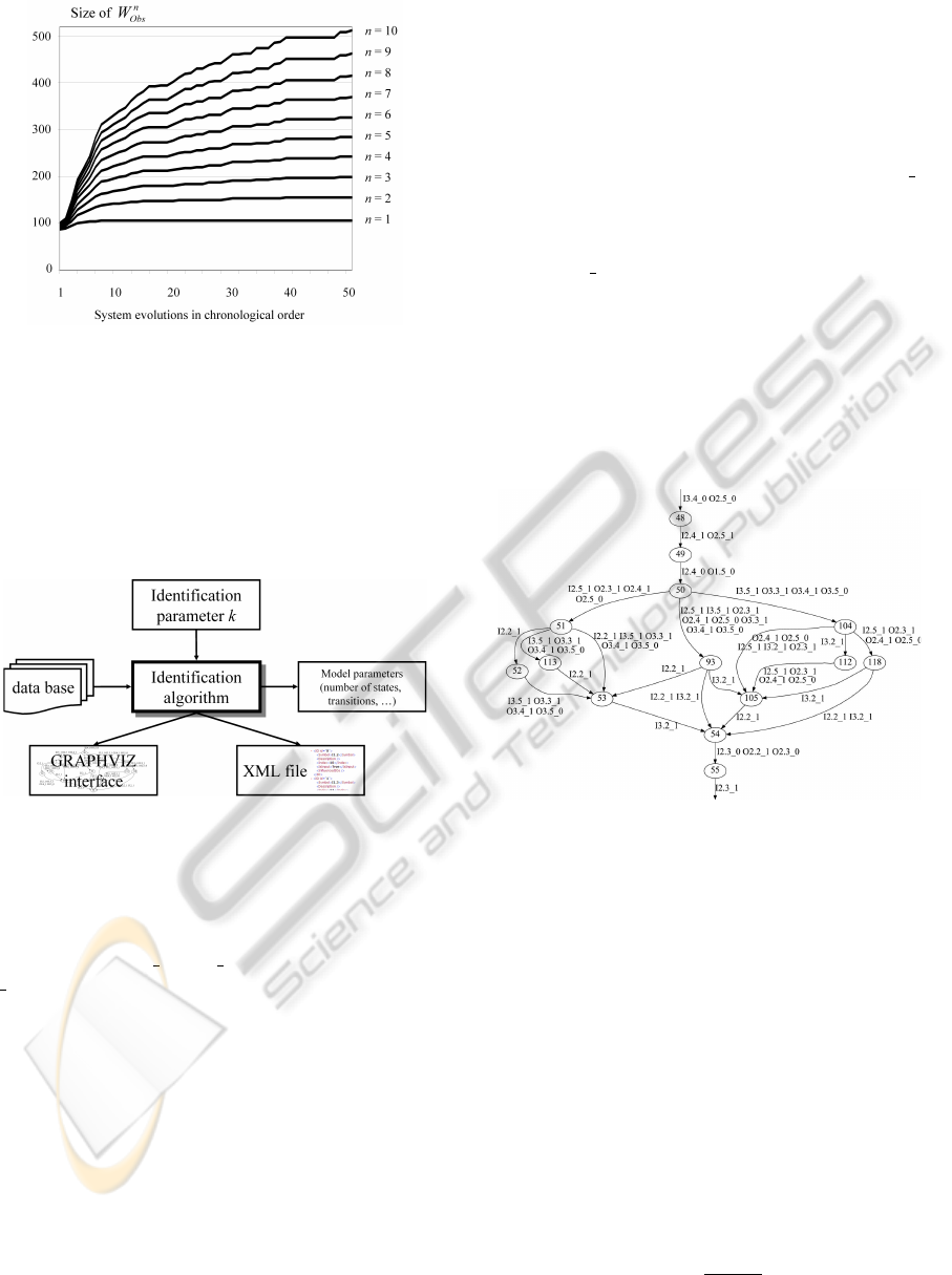
Figure 9: Observed word set for the laboratory system.
an XML-file to use it in other tools such as diagnosis
software (Roth et al., 2009). To visualize the resulting
automaton, an interface to GRAPHVIZ is provided.
The identification of the NDAAO with k = 2 on the
basis of 50 system evolutions took 170 ms on a stan-
dard PC with a 1.79 Ghz CPU and 1.96 GB RAM. The
identified model has 121 states and 162 transitions.
Figure 10: Features of the implemented software.
A part of the identified NDAAO can be seen in
figure 11. Due to space limitations, instead of giv-
ing the complete I/O vector in each state output, only
I/Os changing their value from one state to another
are given (e.g. I2.4 1 O2.5 1 to indicate a rising edge
( 1) of controller Input I2.4 and a rising edge of con-
troller Output O2.5 from state 48 to state 49). Several
examples for the different I/O vector sampling scenar-
ios presented in section 3.1 can be seen in the model.
For the scenario with two controller inputs changing
their value synchronously due to the data collection
process (figure 4), the transition between states 93 and
54 is an example. Both inputs I2.2 and I3.2 change
their value when taking this transition. The transi-
tion from state 48 to 49 is an example for the sec-
ond sampling scenario (figure 5) where the change in
value of an input triggers the change in value of an
output. This transition represents the situation when
the second work arrives at the entrance of the sec-
ond station (position sensor connected to I2.4 changes
its value) and the conveyor of this station is started
(controller output O2.5 is set to 1). Both changes in
value appear at one transition due to the data collec-
tion process as explained in section 3.1. An example
for the third scenario form section 3.1 (figure 6) can
be seen in the state trajectory x
48
→ x
49
→ x
50
. From
state 48 to state 49 the conveyor is started (O2.5 1)
to transport the work piece away from the entrance
position (I2.5). Since it takes at least until the next
PLC cycle to transport the work piece away from the
sensor (I2.5 0 for the falling edge) cause and effect
cannot be seen at once but at some successive transi-
tions. The non-deterministic nature of the identified
NDAAO can also be seen in figure 11: there are sev-
eral ways to go from state 50 to state 55. Being in state
50 the choice of the trajectory is not determined but
taken at random like in the closed-loop DES where
unpredictable physical conditions in the plant lead to
non-deterministic behavior.
Figure 11: Part of the identified NDAAO.
One of the important characteristics of the identi-
fied model is its capability to simulate the complete
original system language (theorem 1). Even if only
a subset of possible I/O vector sequences connecting
the closed-loop system states represented by NDAAO
states 50 and 55 has been observed, the model con-
tains each possible trajectory that can occur when go-
ing from one state to the other as long as no new
word of length k + 1 is produced. If L
k+1
Orig
= L
k+1
Obs
,
the model is capable of exhibiting words of length
k + n although these words have not been seen be-
fore. This capability comes at cost of also exhibit-
ing words that have not and probably will not be ob-
served (w
k+n
/∈ L
k+n
Orig
). To get some information of
the amount of words which are created without hav-
ing been observed, the coefficient
C
n
B
=
|L
n
Ident
|
|L
n
Obs
|
is a useful indicator. The presentation of the coeffi-
IDENTIFICATION OF DISCRETE EVENT SYSTEMS - Implementation Issues and Model Completeness
79

cient in figure 12 describes the relation between the
identified and the observed language of an automa-
ton identified with k = 2. For n = k + 1, the model
strictly creates the observed language L
k+1
Obs
. It can be
seen that for larger values of n the automaton gener-
ates a larger language than L
n
Obs
. A certain part of the
additionally created words is probably not part of the
original system language which may lead to a need for
specific precautions in some model based techniques
like diagnosis. However, from theorem 1 it is clear
that each word with length n ≥ k + 1 of the original
language not observed so far is part of the identified
language. In the case of model based diagnosis for
example, this allows stating that there will be no false
alerts using the identified automaton as fault-free ref-
erence model (Roth et al., 2009).
Figure 12: Coefficient of identified and observed language.
6 CONCLUSIONS
In this paper practical implications of identification
of closed-loop discrete event systems have been ad-
dressed. It has been shown how the necessary data
can be obtained in the case of industrial closed-loop
systems. For many model-based techniques it is cru-
cial to have a model of the complete system behav-
ior. For the identification algorithm of (Klein, 2005) it
has been proved that the identified automaton is sim-
ulates the original system language of arbitrary length
if some conditions concerning the observed system
language hold.
REFERENCES
Biermann, A. and Feldman, J. (1972). On the synthesis of
finite-state machines from the sample of their behav-
ior. IEEE transactions on computers, 21:592–597.
de Smet, O., Denis, B., Lesage, J.-J., and Roussel, J.-M.
(2001). Dispositif et procd d’analyse de performances
et d’identification comportementale d’un systme in-
dustriel en tant qu’automate vnements discrets et fi-
nis. Technical report, French Patent 01 110 933.
Dotoli, M., Fanti, M. P., and Mangini, A. M. (2006). On-
line identification of discrete event systems: a case
study. In 2006 IEEE international conference on au-
tomation science and engineering, pages 405–410.
Fanti, M. P. and Seatzu, C. (2008). Fault diagnosis and iden-
tification of discrete event systems using petri nets.
In Proceedings of the 9th International Workshop on
Discrete Event Systems, Gtebor, Sweden, pages 432–
435.
Giua, A. and Seatzu, C. (2005). Identification of free-
labeled petri nets via integer programming. Proceed-
ings of the 44th IEEE Conference on Decision and
Control, and the European Control Conference 2005
Seville, Spain, December 12-15, 2005, pages 7639–
7644.
Klein, S. (2005). Identification of Discrete Event Systems
for Fault Detection Purposes. Shaker Verlag.
Klein, S., Litz, L., and Lesage, J.-J. (2005). Fault detec-
tion of discrete event systems using an identification
approach. In Proceedings of the 16th IFAC World
Congress, pages CDROM paper n02643, 6 pages.
Machado, J., Denis, B., and Lesage, J. J. (2006). A generic
approach to build plant models for DES verification
purposes. In Proceedings of the 8th international
workshop on discrete event systems, pages 407–412.
Meda-Campana, M. and Lopez-Mellado (2005). Identifica-
tion of concurrent discrete event systems using petri
nets. 2005 IMACS: Mathematical Computer, Mod-
elling and Simulation Conference.
Roth, M., Lesage, J.-J., and Litz, L. (2009). An FDI
method for manufacturing systems based on an iden-
tified model. In Proceedings of the 13th IFAC Sympo-
sium on Information Control Problems in Manufactur-
ing, INCOM’09, pages 1389 – 1394, Moscow, Russia.
IFAC.
Sampath, M., Sengupta, R., Lafortune, S., Sinnamohideen,
K., and Teneketzis, D. (1996). Failure diagnosis using
discrete-event models. IEEE transactions on control
systems technology, 4(2):105–124.
ICINCO 2010 - 7th International Conference on Informatics in Control, Automation and Robotics
80
