
PREDICTION OF TEMPERATURE INSIDE A REFRIGERATED
CONTAINER IN THE PRESENCE OF PERISHABLE GOODS
Javier Palafox-Albarrán, Reiner Jedermann and Walter Lang
Institute of Microsensors Actuators and Systems (IMSAS), University of Bremen
Otto Hahn Allee NW1, D-28359 Bremen, Germany
Keywords: System Identification, Temperature, Organic Heat, Feedback-hammerstein.
Abstract: This paper presents an alternative method to predict the temperature profile in a spatial point of the interior
of a refrigerated container with the aim of improving the logistics of perishable goods. A SISO gray-box
model in which the organic heat is represented by a non-linear feedback system and the cooling process
represented by a linear system is proposed. Parameter adaptation and prediction algorithms for the model
are modified to reduce the matrix dimensions, implemented in Matlab and applied to experimental data for
validation. Apart from being highly accurate, the predictions comply with the desired figures of merit for
the implementation in wireless sensor nodes, such as high robustness against quantization and enviromental
noise. Simulation results concludes that if the cargo emits organic heat, the proposed model is faster and
more accurate than the linear models.
1 INTRODUCTION
Research has been done in the past to estimate the
temperature profile inside refrigerated containers.
Several options have been investigated:
mathematical approaches as presented in (Shaik,
2007), K-ε models as proposed in (Rouaud, 2002),
and several numerical models as reviewed in
(Smale, 2006). With the exception of
(Moureh,2004), in which the effect of the pallets is
considered; usually the focus is put on the cold air
flow as the main factor governing the temperature
pattern inside a container and the effects due the
cargo presence is sub estimated.
To take into account the effect of the cargo in the
temperature, in (Babazadeh, 2008) it is proposed the
use of wireless sensor nodes (WSN) to measure the
ambient parameters in the surroundings of a spatial
point of interest and the use of system identification
to estimate the parameters of a linear Multi-Input
Single-Output (MISO) system. It concluded that in
order to have a good estimation, it is necessary to
have a high number of training samples and many
inputs to the system.
In this paper an alternative Single-Input Single-
Output (SISO) grey-box model is presented to
predict the temperature inside the container under
the presence of perishable goods with the aim of
reducing the complexity and preserving the
accuracy. The proposed model provides a
meaningful description of the factors involved in the
physical system including the effect of transporting
living goods such as fruits and vegetables. The
starting point is based on the physical relations;
subsequently, a tuning parameter for the specific
case of bananas is found by simulations.
2 MODEL OF THE SYSTEM
The factors affecting the temperature distribution
inside a refrigerated container are illustrated in
Figure 1. The cold air flows from bottom to top
through the gratings in the floor and through the
spaces between the pallets, and eventually it is
drawn off the channel between the pallets and the
container ceiling.
A naive representation of the container can be
done by a SISO linear dynamic system in which the
input is the air supply and the output is the spatial
20
Palafox-Albarrán J., Jedermann R. and Lang W. (2010).
PREDICTION OF TEMPERATURE INSIDE A REFRIGERATED CONTAINER IN THE PRESENCE OF PERISHABLE GOODS.
In Proceedings of the 7th International Conference on Informatics in Control, Automation and Robotics, pages 20-27
DOI: 10.5220/0002880100200027
Copyright
c
SciTePress

Temperature
o
C
Yellow
Green
Heat
W/ Ton
3
00
2
00
1
00
point of interest. However, in reality it is only a
simple model of the main contributor to the
temperature pattern, the air flow. Several other
factors affect the speed of the cooling down.
To improve the accuracy of the model, other
contributors are considered as well: first is the heat,
produced by respiration of living goods such as
fruits and vegetables; second is the thermal loss,
affecting the correct cooling of the goods; finally,
unpredictable temperature variations due to highly
changing external climatic conditions during
transportation.
Figure 1: Factors affecting the temperature inside a
refrigerated container.
The linear SISO black-box model representing
the air flow is represented mathematically by a
linear dynamic system H, which in the discrete
domain is given by the Equation 1.
1
=
1
1
1
(1)
Where
and
are the orders of the system
polynomials,
1
,
1
are the polynomial
coefficients, and is the delay operator in discrete
domain.
An attenuator, α ,models the isolation loses of
the air supply temperature and is modeled to affect
the input of the dynamic system. The external
climatic conditions are unknown in advance,
therefore considered a statistical process. The output
of the Moving Average (MA) process, which is in
fact white noise (WN) filtered by the filter C
represented in Equation 2 added to the output of the
dynamic system, models them.
(
1
) = 1 +
1
1
+ +
(2)
To model the organic heat, it is necessary to use
experimental data. Figure 2 (Mercantila, 1989)
shows a family of curves for organic heat in the case
of bananas. A proportional relationship between of
the organic heat and the rippening state is observed.
Equation 3 represents the organic heat relation
with respect to the temperature.
is the heat
production in Watts, is a constant which is fixed
for a certain type of fruit and rippening-state in 1/
O
C,
is the fruit temperature in
O
C, and is a scaling
factor which depends of the amount of food and is
given in kilograms.
=
(3)
Figure 2: Heat Production of bananas.
Finally, the block diagram to represent the input-
output relations of all the factors is built. It is shown
in Figure 3. The air flow dynamics are represented
as a feed-forward block as it is the most important
contributor. The isolation losses affect the correct
cooling of the goods before the dynamic system and
the noise effect has an additive effect on the output.
The contribution of the organic heat depends on
the cooling temperature inside the container.
Simultaneously, it has a small additive effect in the
input of the linear dynamic system as the air flows
through the pallets and is slightly warmed. It is
represented by a static exponential feedback. The
resulting block diagram, in which a linear dynamic
system has a non-linear feedback corresponds to a
Feedback-Hammerstein (FH) configuration (Guo,
2004).
Figure 3: Model of the system.
Organic heat
Isolation losses
Disturbances
PREDICTION OF TEMPERATURE INSIDE A REFRIGERATED CONTAINER IN THE PRESENCE OF
PERISHABLE GOODS
21

3 PARAMETER ADAPTATION
ALGORITHM
In (Guo, 2004) a Parameter Adaptation Algorithm
(PAA) was developed to identify the parameter-set
of a FH system. It uses an intermediate variable
and converts the non-linear system into a pseudo-
linear one. Its principal advantage is that the
conventional recursive matrix-based linear system
identification algorithms as those presented in
(Landau, 2005) can be applied to estimate the
parameter matrix . The recursive form of those
algorithm is given by Equation 4. Where () is the
prediction error as described in Equation 5, P(t+1)
is an adaptation matrix to perform the minimization
of ε using Recursive Least Squares method, and φ(t)
is the observation matrix that contains the input and
the output data.
+ 1
in Equation 6 is the so
called Forgetting Factor (FF).
(t+1)=(t)+(P
t + 1
φ(t))
()
(4)
() = () ()
φ(t-1)
(5)
P(t+1)=
()()φφ
(
()
φ
φ+(+1)
)
(+1)
(6)
+ 1
=
+ 1
(7)
Guo considers the non-linearity as a polynomial
of order l as shown in Equation 8; however, the
dimensions of the matrices in the algorithm would
be significantly too large to be applied in platforms
where power consumption is an important figure of
merit.
y
=
y
k
=0
(t)
(8)
To reduce the dimensions of the matrices, was
proposed the use of the exponential Equation in
Equation 3 instead. γ is to be determined and it
remains constant, while β is a parameter to be
identified as it depends on the amount of fruit being
transported. The linear term of the Equation 8 needs
to be extracted to be included in the polynomial
1
of the equivalent SISO pseudo-linear
system. Expanding it into a Taylor series and
rearranging, the summation of the non-linear
coefficients of the exponential function can be
calculated using Equation 9. The non-linear
coefficients and an offset are on the left hand of the
equation.
()
!
∞
=2
+1 =
()
()
(9)
The equivalent pseudo-linear system for an
exponential non-linearity is shown in Equation 10.
1
y
t
=
1
+
1
1
() +
1
1
+
1
(10)
The resulting coeficients of the polynomials
(
1
) and
1
are given by Equation 11 and
12.
=
()
(11)
1
=
2
2
+ +
(12)
And the intermediate variable is shown by
Equation 13.
=
1
+ (
()
())
(13)
The choice of the forgetting factor in the
algorithm is often critical. In theory, it must be one
that converges. On the other hand, if it is less than
one the algorithm becomes more sensitive and the
estimated parameter changes quickly making the
convergence faster. A more complex solution is to
allow it to vary with time, lower than one at the
beginning but tending to one.
Figure 4: Types of forgetting factors.
Figure 4 illustrates three different types of FF. The
first case is obtained by making
, and
in
Equation 7 equal to one. It is called Decreasing Gain
(DG). In the second case, the Constant Forgetting
Factor (CFF)
is set to a value smaller than one
and
set to one. Finally, the Variable Forgetting
Factor (VFF) uses a value of
smaller than one
and recalculates
for each iteration.
ICINCO 2010 - 7th International Conference on Informatics in Control, Automation and Robotics
22
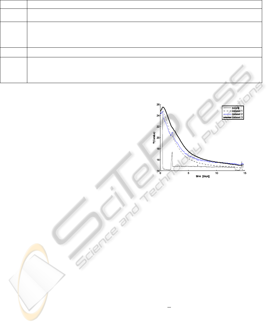
Table 1: Elements of the elements in the algorithm matrices.
Symbol
Arrangement of the elements into the matrices
φ(t)
···
+ 1
,
1
, (
),
1
. . .
),
···
+ 1
()
1
,
1
,
1
,
2
1
1
,
1
(t)
+ 1
,
, (
),
1
. . .
)
()
1
,
1
,
1
,
2
1
1
4 PREDICTION ALGORITHM
The predictions are made using the estimated
parameters in the model. Figure 5 shows
experimental data sets from a container transporting
bananas. It can be observed how the air supply is
kept constant after some days. For the prediction
algorithm, () is set to the value of the last sampled
input temperature of the parameter adaptation
process. Similarly, the initial predicted output value
is set to the last acquired value of the output.
Equation 14 to 17 describes the prediction
algorithm. m is the number of iterations used for the
PAA.
=
(14)
() =
(15)
()=
(m) φ
(t-1)
(16)
=
1
+ (
()
())
(17)
5 DETERMINATION OF γ
In considering a linear system, an exponential
discrete time decaying system like the one presented
in Figure 5 can be described as of the order of one
with its unique pole on the real positive axis. The
closer the pole to one the higher the delay of the
system.
Figure 5: Banana data sets.
To find a trustworthy parameter that
characterizes the respiration heat of bananas. The
presented Feedback-Hammerstein model of linear
order one and the FH parameter adaptation and
prediction algorithms are run using given
experimental data sets. The Mean Squared Error
(MSE) of the prediction over n samples, equivalent
to fifteen days, is stored for several values of γ and
fixed number of training days. If the stored values of
the MSE are plotted, the local minimums are
determined by the observation of the MSE vs. γ
curves. In Figure 6, it can be seen that in the above
mentioned plot for five days of training and for the
data set 1, a local minimum exists for a value γ of
0.0587.
=
1
(
)
2
=
(18)
PREDICTION OF TEMPERATURE INSIDE A REFRIGERATED CONTAINER IN THE PRESENCE OF
PERISHABLE GOODS
23
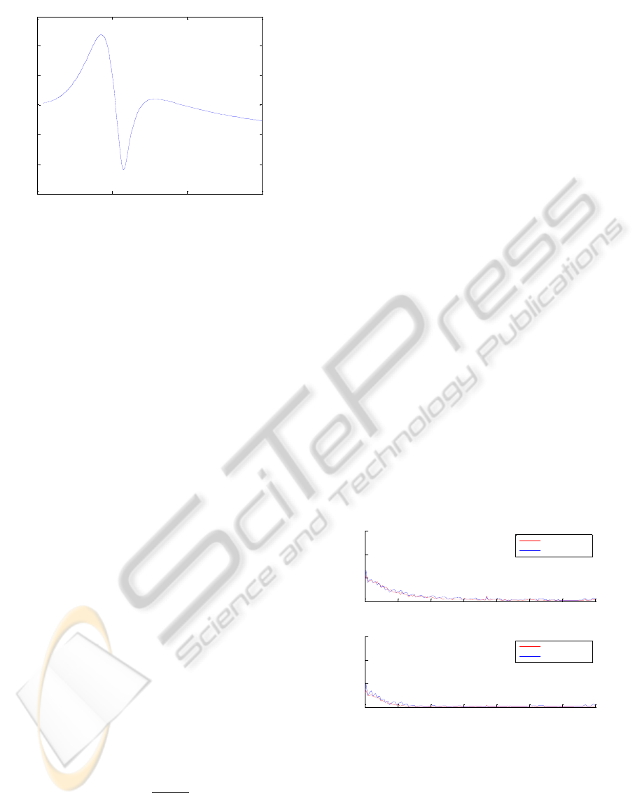
Figure 6: Prediction accuracy vs. γ.
6 RESULTS
For validation of the model and algorithms several
figures of merit are considered. The accuracy and
the speed of convergence are of paramount
importance; however, quantization and noise
robustness are also highly desirable for
implementation in a WSN. Only the linear orders of
one and two are considered to avoid computation of
complex conjugate poles that would characterize
oscillations.
To observe the speed of convergence and the
accuracy of the predictions with respect to the
number of training days, parameter estimation and a
prediction in Matrix form are done (See Table 1) for
a fixed number of training days. Subsequently, MSE
vs. Training days graphs are plotted. Assuming a
quantization level of 0.2
O
C, a Matlab script was
written to assign the nearest value of the
quantization grid to the input and the output datasets.
The results of the predictions using the quantized
datasets are overlapped with the results of non-
quantized.
Similarly, to determine the noise robustness,
MSE versus the signal to noise ratio (SNR) is
plotted. Several noise levels of white noise were
added to the output of the data set 1, and the
resulting signals were applied to PAA and prediction
algorithms with fixed number of training days.
SNR(dB)=10log
(19)
Simulations were done for two types of data sets.
First, the experimental data of bananas were used to
include the presence of organic heat. Secondly, the
data sets corresponding to a cheese experiment,
which does not present organic heat, were
considered. A summary of all simulation results is
presented on Table 2.
6.1 FH vs. Linear Models
in the Presence of Organic Heat
From the simulations it is observed in Figures 7 and
8 that if linear methods are applied to the banana
datasets, the accuracy of the results for different
sensor positions of are not sufficient. Quantization
robustness is improved with the linear order of one
and the speed of convergence is better using CFF. In
the best of cases acceptable prediction accuracy can
only be achieved after more than five days of
training.
It is also observed in Figures 8 and 9 that FH
identification algorithms are the best to achieve fast
convergence speeds. In the best cases, less than 3
days of training is sufficient to achieve good
predictions. However, the plots are made for the data
from three days onwards to avoid the visualization
of the effects in MSE due to the set point variations
in the reefer supply temperature. Linear system
orders of one are in all cases better than order of
two, both in the speed of convergence and the
quantization robustness. Decreasing Gain must be
optimal to preserve the accuracy and the
quantization robustness.
Figure 7: ARX of order one in the presence of organic
heat.
Concerning the noise models, results of the
simulation of Feedback-Hammerstein with MA
process are worse than when modeled as white noise
(WN). It affects the accuracy and the quantization
robustness
0 0.05 0.1 0.15
0
0.2
0.4
0.6
0.8
1
MSE
Values of
MSE of FH ARX PAA with respect to gamma
3 4 5 6 7 8 9 10
0
1
2
3
Training Days
MSE
Order of one and DG
Non-quantized
Quantized
3 4 5 6 7 8 9 10
0
1
2
3
Training Days
MSE
Order of one and CFF
Non-quantized
Quantized
ICINCO 2010 - 7th International Conference on Informatics in Control, Automation and Robotics
24
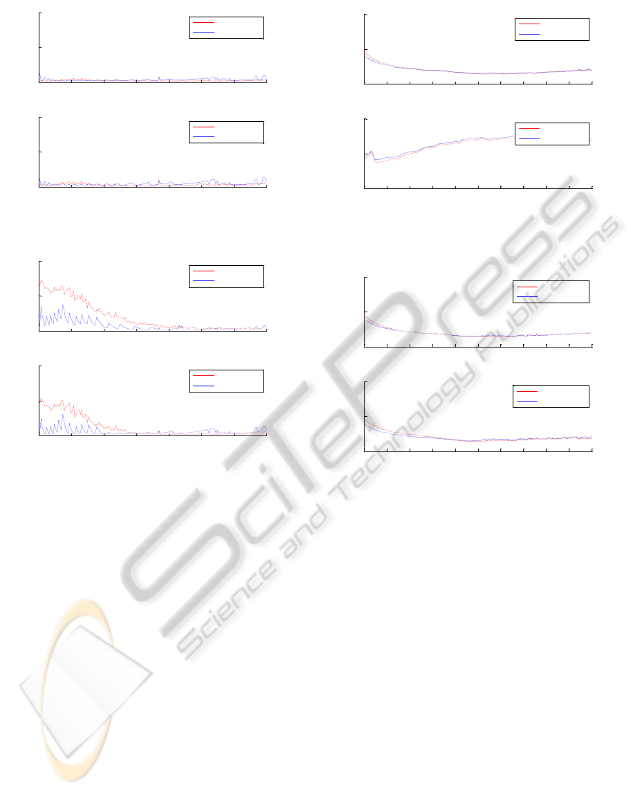
Figure 8: FH of order one in the presence of organic heat.
Figure 9: FH of order two in the presence of organic heat.
6.2 FH vs. Linear Models
in the Absence of Organic Heat
In the case of cheese data set, the linear methods
accuracy results are better than that of the Feedback-
Hammerstein as can be observed in Figure 10.
Modeling noise as white gives better quantization
robustness than modeling it as MA process.
The use of forgetting factors does not have a big
impact in the results of ARX predictions; however,
Constant Forgetting Factor is slightly better for
ARMAX predictions. Linear orders do not affect
the simulated predictions, but an order of two is
selected because it can model more accurately if the
behavior of the system is not purely decaying.
Figure 10: Comparison of FH and linear methods in the
absence of organic heat.
Figure 11: Comparison of linear methods with MA and
WN models.
6.3 Noise Robustness
The noise was added to validate FH and linear
models; also for both of them the accuracy is
compared with and without the MA model.
Maximum Signal-to-Noise Ratio to obtain a good
prediction is observed to be around 43 dB for all of
them with the exception of ARX which has a
maximum value of 47 Decibels as shown in Table 2.
6.4 Prediction Improvement
The described approach was originally developed
based on an experiment in 2008 with records for 3
sensors (data set A). Two new data sets with 16
sensors each, which were recorded in 2009
(Jedermann, 2010) in two separate containers (data
set B and C), were used to cross validate the
approach.
3 4 5 6 7 8 9 10
0
0.5
1
Training Days
MSE
Order of one and DG
Non-quantized
Quantized
3 4 5 6 7 8 9 10
0
0.5
1
Training Days
MSE
Order of one and CFF
Non-quantized
Quantized
3 4 5 6 7 8 9 10
0
0.5
1
Training Days
MSE
Order of two and DG
Non-quantized
Quantized
3 4 5 6 7 8 9 10
0
0.5
1
Training Days
MSE
Order of two and CFF
Non-quantized
Quantized
3 3.5 4 4.5 5 5.5 6 6.5 7 7.5 8
0
0.5
1
Trainining Days
MSE
Linear ARX of order of one
Non-quantized
Quantized
3 3.5 4 4.5 5 5.5 6 6.5 7 7.5 8
0
0.5
1
Trainining Days
MSE
FH of linear order of one
Non-quantized
Quantized
3 3.5 4 4.5 5 5.5 6 6.5 7 7.5 8
0
0.5
1
Time (Days)
MSE
Linear ARX of order of two
Non-quantized
Quantized
3 3.5 4 4.5 5 5.5 6 6.5 7 7.5 8
0
0.5
1
Time (Days)
Average Error
Linear ARMAX of order of two
Non-quantized
Quantized
PREDICTION OF TEMPERATURE INSIDE A REFRIGERATED CONTAINER IN THE PRESENCE OF
PERISHABLE GOODS
25
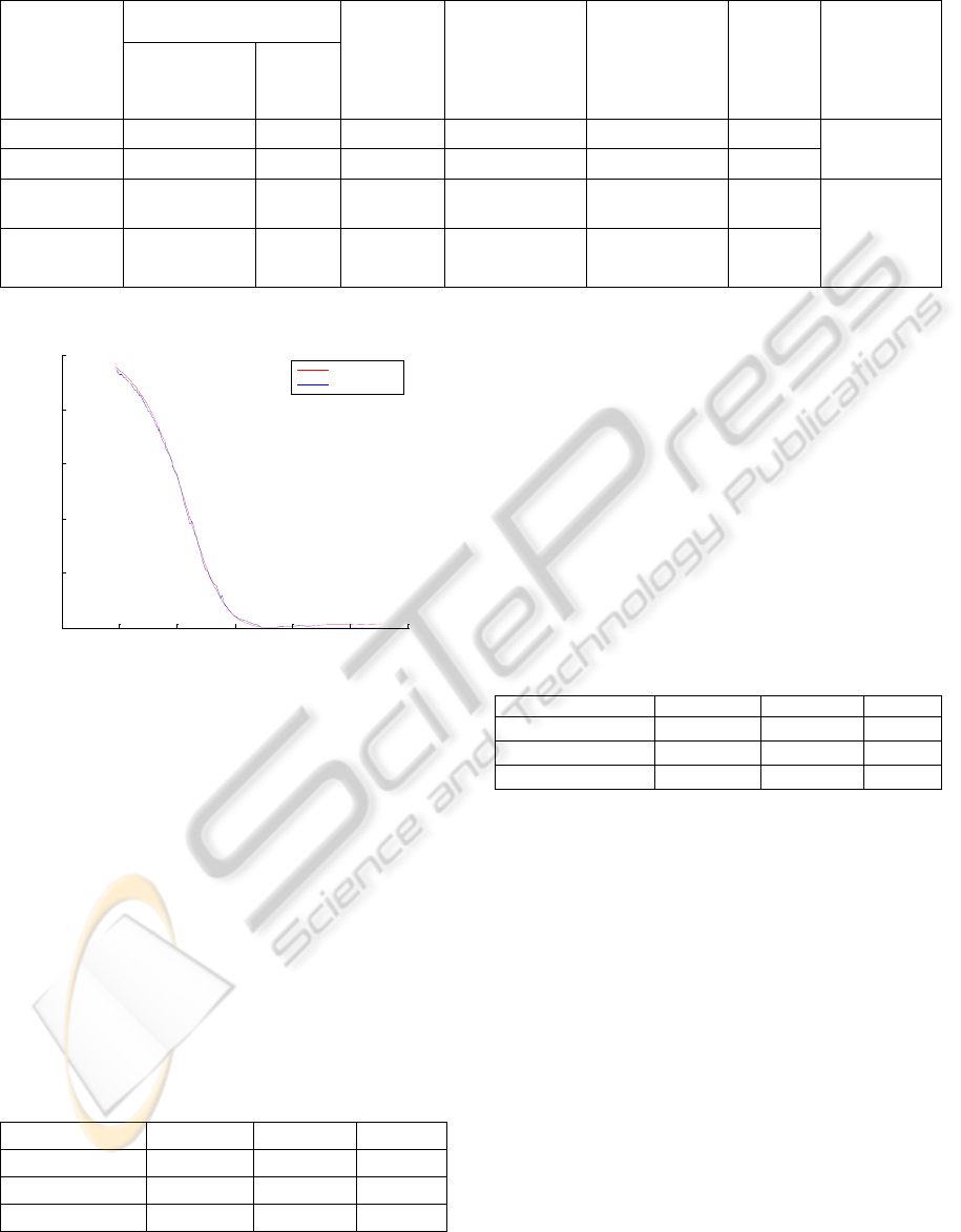
Table 2: Summary of simulation results.
Accuracy
Number
of
matrix
elements
Convergence
speed
Quantization
Robustness
Critical
SNR
Estimation
for linear
dataset
Best
Forgetting
Factor
Best
Linear
order
ARX
CFF
2
3
Bad
Good
47dB
Good
ARMAX
CFF
2
3 +
Bad
Bad
43 dB
FH and WN
model
DG
1
3
Good
Good
43 dB
Bad
FH and MA
model
DG
1
3 +
Good
Bad
43 dB
Figure 12: Noise Robustness for FH method
FH algorithm of linear order of one was applied
to all data sets; neither quantization nor forgetting
factor is used. For the initial parameter settings, the
pole and zero of the feed-forward linear system was
set to 0.9 and 0.0; β was set to 2.
The previously obtained value of γ equal to
0.0587 is used to predict the temperature inside the
containers for many spatial positions. The results are
compared to the predictions for the datasets shown
in Figure 5 and resumed in Table 3. A good average
is observed for the three containers; however, in
some positions the predictions are not as accurate as
is observed in the Maximum column.
Table 3: MSE prediction results for a unique value of γ.
Container/Result
Maximum
Minimum
Average
Data set A
0.1893
0.0173
0.0778
Data set B
1.4558
0.0550
0.4130
Data set C
0.8888
0.0101
0.2798
A second approach is to select γ according to the
position of the pallets inside the container. The
method to find γ, described previously, is applied to
all the new container datasets.
It is observed that an improvement in the
accuracy of the predictions can be made if two
different values of γ are selected: one for pallets
close to the door-end, and one for pallets close to the
reefer supply. In Table 4 it is resumed the prediction
results if values of 0.0525 and 0.055 are set
respectively.
Table 4: MSE prediction results for values of γ according
to the position inside the container.
Container/Result
Maximum
Minimum
Average
Data set A
0.1893
0.0173
0.0778
Data set B
0.4767
0.0279
0.0946
Data set C
0.5747
0.0201
0.1743
7 CONCLUSIONS
A model to represent the factors affecting the
temperature inside a refrigerated container
transporting perishable goods was proposed. It
models the effect of organic heat using a static non-
linear feedback system, the refrigeration by a linear
dynamic feed-forward system, and the disturbances
by stochastic processes. This complex model can
provide an accurate description of the factors
involved in the physical system.
The selected identification method was adapted
specifically to reduce the dimensions of the
matrices. The non-linear exponential function is
used instead of a polynomial to preserve the
simplicity of the parameter adaptation and the
prediction algorithms. The disadvantage of the
10 20 30 40 50 60 70
0
5
10
15
20
25
Signal to Noise Ratio(dB)
MSE
FH ARX Prediction Error vs SNR
Non-quantized
Quantized
ICINCO 2010 - 7th International Conference on Informatics in Control, Automation and Robotics
26

simplification is that depending on the kind of fruits
to be transported, it is required to tune the algorithm
by a correct selection of γ which has to be known in
advance. An improvement can be observed in the
accuracy of the predictions if γ is set according to
the position of the pallets inside the container.
From the simulation results it is concluded that
the FH identification algorithm is efficient when the
cargo emits organic heat. The method of FH of order
1 is optimal to achieve all figures of merit. It makes
accurate predictions only after three days of training
and maintains low dimensions of matrices.
However, if the linear method is applied to the
banana datasets, a comparable accuracy can only be
achieved after more than five days of training. Also,
it is concluded that when the goods to transport are
free of organic heat, such as in the case of cheese, it
is preferable to use a linear system instead.
ACKNOWLEDGEMENTS
The authors would like to express their gratitude to
Prof. Rainer Laur, Dirk Hentschel, Mehrdad
Babazadeh, and Chanaka Lloyd for all their help.
This research was supported by the German
Research Foundation (DFG) as part of the
Collaborative Research Centre 637 “Autonomous
Cooperating Logistic Processes”. Further project
information can be found at
www.intelligentcontainer.com.
REFERENCES
Babazadeh, M., Kreowski, H.-J., Lang, W, 2008. Selective
Predictors of Environmental Parameters in Wireless
Sensor Networks. In International Journal of
Mathematical Models and Methods in Applied
Sciences Vol.2, pages 355-363.
Guo, F., 2004. A New Identification Method for Wiener
and Hammerstein System. Ph.D. Thesis, Institut für
Angewandte Informatik Forschungzentrum Karlsruhe.
Karlsruhe.
Jedermann, R., Becker, M., Görg, C., Lang, W., 2010.
Field Test of the Intelligent Container, In European
Conference on Wireless Sensor Networks
EWSN2010, 16-19 February 2010 in Coimbra,
Portugal.
Landau, I.D., Zito G., 2006. Digital Control Systems:
Design, identification and implementation. Springer.
London, 1st edition.
Mercantila. 1989. Guide to food transport: fruit and
vegetables. Mercantila Publ. Copenhagen.Moureh J.,
Flick, D., 2004. Airflow pattern and temperature
distribution in a typical refrigerated truck
configuration loaded with pallet. In International
Journal of Refrigeration, V. 27, Issue 5, pages 464-
474.
Palafox J., 2009. Prediction of temperature in the transport
of perishable goods based in On-line System
Identification. M.Sc. Thesis, University of Bremen.
Bremen.
Rouaud, O., Havet, M., 2002. Computation of the airflow
in a pilot scale clean room using K-ε turbulence
models, In International Journal of Refrigeration, Vol.
25, Issue 3, pages 351-361.
Shaikh, N. I., Prabhu, V., 2007.Mathematical modeling
and simulation of cryogenic tunnel freezers. In Journal
of Food Engineering, Vol. 80, Issue2, pages 701-710.
Smale, N. J., Moureh,J., Cortella, G., 2007.A review of
numerical models of airflow in refrigerated food
applications. In International Journal of Refrigeration,
Vol. 29, Issue 6, pages 911-930.
LIST OF ABBREVIATIONS
ARMAX
ARX
CFF
DG
FF
FH
MA
MSE
PAA
WN
WSN
Auto Regressive Moving Average
with External input.
Auto Regresive with External input.
Constant Forgetting Factor
Decreasing Gain
Forgetting Factor
Feedback Hammerstein
Moving Average
Mean Squared Error
Parameter Adaptation
AlgorithmWhite Noise
Wireless Sensor Node
PREDICTION OF TEMPERATURE INSIDE A REFRIGERATED CONTAINER IN THE PRESENCE OF
PERISHABLE GOODS
27
