POSITION ESTIMATION OF MOBILE ROBOTS CONSIDERING

CHARACTERISTIC TERRAIN PROPERTIES

Michael Brunner, Dirk Schulz

Department of Unmanned Systems, Fraunhofer-Institute FKIE, Wachtberg, Germany

Armin B. Cremers

Department of Computer Science, University of Bonn, Bonn, Germany

Keywords:

Mobile robots, Position estimation, Terrain classiﬁcation, Machine learning.

Abstract:

Due to the varying terrain conditions in outdoor scenarios the kinematics of mobile robots is much more

complex compared to indoor environments. In this paper we present an approach to predict future positions of

mobile robots which considers the current terrain. Our approach uses Gaussian process regression (GPR) mod-

els to estimate future robot positions. An unscented Kalman ﬁlter (UKF) is used to project the uncertainties

of the GPR estimates into the position space. The approach utilizes optimized terrain models for estimation.

To decide which model to apply, a terrain classiﬁcation is implemented using Gaussian process classiﬁcation

(GPC) models. The transitions between terrains are modeled by a 2-step Bayesian ﬁlter (BF). This allows us

to assign different probabilities to distinct terrain sequences, while taking the properties of the classiﬁer into

account and coping with false classiﬁcations. Experiments showed the approach to produce better estimates

than approaches considering only a single terrain model and to be competitive to other dynamic approaches.

1 INTRODUCTION

The kinematics of mobile robots in outdoor scenarios

is much more complex than in indoor environments

due to the varying terrain conditions. Therefore, truly

reliable velocity controls for robots which are able to

drive up to 4 m/s or even faster (e.g. Figure 1) are hard

to design. The drivability is primarily determined by

the terrain conditions. Thus, we developed a machine

learning system which predicts the future positions of

mobile robots using optimized terrain models.

In this paper we present a Gaussian processes

(GPs) based method for estimating the positions of

a mobile robot. Our approach considers the differ-

ent terrain conditions to improve prediction quality.

Gaussian process regression (GPR) models are uti-

lized to estimate the translational and rotational ve-

locities of the robot. These estimated velocities are

transferred into the position space using an unscented

Kalman ﬁlter (UKF). By projecting the uncertainty

values of the GPR estimates onto the positions, the

UKF enables us to also capitalize the GPR uncertain-

ties. To distinguish the different terrains the robot is

traversing, we classify the spectrums of vertical accel-

erations using Gaussian process classiﬁcation (GPC).

The transitions between terrains are modeled by a 2-

step Bayesian ﬁlter (BF). This allows us to assign dif-

ferent probabilities to distinct terrain sequences, as we

incorporate the properties of the classiﬁer.

The remainder of this paper is organized as fol-

lows: Related work is presented in Section 2. In Sec-

tion 3 we explain GPs. In Section 4 we describe our

dynamic approach. Experiments are shown in Sec-

tion 5. We conclude in Section 6.

2 RELATED WORK

Several works study Gaussian processes (GPs)

and their application to machine learning prob-

lems. A detailed view is provided by Rasmussen

and Williams (Rasmussen and Williams, 2005).

Other works are Williams (Williams, 2002), and

MacKay (MacKay, 1998).

There is a lot of research on prediction of po-

sitions or trajectories of mobile robots. Many dif-

ferent systems are proposed, like a stereo-vision ap-

proach (Agrawal and Konolige, 2006), probability

Brunner M., Schulz D. and B. Cremers A. (2010).

POSITION ESTIMATION OF MOBILE ROBOTS CONSIDERING CHARACTERISTIC TERRAIN PROPERTIES.

In Proceedings of the 7th International Conference on Informatics in Control, Automation and Robotics, pages 5-14

DOI: 10.5220/0002880200050014

 SciTePress

Figure 1: The experimental Longcross platform Suworow.

networks (Burgard et al., 1996) or an approach us-

ing a particle ﬁlter combined with a Monte-Carlo

method (Thrun et al., 2000). In (Seyr et al., 2005) arti-

ﬁcial neural networks (ANN) are employed to build a

model predictive controller (MPC). The current pre-

diction error is considered to improve the quality of

the velocity estimations. Another least-square sup-

port vector machine (LS-SVM) based controller ad-

justs it’s data model iteratively by removing the least

important data point from the model when adding a

new point (Li-Juan et al., 2007).

Similar to the work presented here, GPs are used

by Girard et al. (Girard et al., 2003) to make predic-

tions several time steps ahead. The uncertainty of the

previous step is integrated in the regression to track

the increasing uncertainty of the estimation. Hence,

the uncertainty value of the GP is the accumulated

uncertainty of the previous time series. In contrast,

we are able to relate the Gaussian uncertainties by us-

ing an UKF. A similar approach has been suggested

by (Ko et al., 2007b), and (Ko et al., 2007a). They

estimated the trajectory of an autonomous blimp by

combining GPR with an UKF or ordinary differential

equations (ODE), respectively. Localization of wire-

less devices, like mobile telecommunication devices

or mobile robots is solved by modeling the probability

distribution of the signal strength with GPs integrated

in a BF (Ferris et al., 2006).

Several works employ information about the cur-

rent terrain conditions to improve the navigation sys-

tems of mobile robots. One intuitive approach is to

distinguish between traversable and non-traversable

terrain (Dahlkamp et al., 2006), (Rasmussen, 2002).

In contrast to the binary separation, Weiss et al.

(Weiss et al., 2006) are using a SVM to classify

the vertical accelerations and hence the terrain type.

Using spectral density analysis (SDA) and principal

component analysis (PCA) Brooks et al. (Brooks

et al., 2005) concentrate on the vibrations a mobile

robot experiences while driving. The preprocessed

data records are categorized through a voting scheme

of binary classiﬁers. Another way to analyse the driv-

ing conditions is to measure the slippage (Iagnemma

and Ward, 2009), (Ward and Iagnemma, 2007).

Kapoor et al. (Kapoor et al., 2007) are using GPs

with pyramid-match kernels to classify objects from

visual data. Urtasun and Darrell (Urtasun and Darrell,

2007) chose a GP latent variable model to achieve a

better classiﬁcation by reducing the input dimension.

Although many works concentrate on position es-

timation as well as terrain classiﬁcation, none com-

bined GPR and GPC to solve both problems at once

for a velocity controller of high speed outdoor robots.

3 GAUSSIAN PROCESSES

GPs are applicable to regression as well as classiﬁca-

tion tasks. In contrast to other methods GPs do not

have any parameters that have to be determined man-

ually. However, the kernel function affects the prop-

erties of a GP essentially and must be chosen by hand.

The parameters of of GPs can be automatically opti-

mized using the training data. Furthermore, GPs pro-

vide uncertainty values additionally to the estimates.

These properties makes GPs attractive for regression

and classiﬁcation task like position estimation and ter-

rain classiﬁcation. However, a drawback of GPs is

their running time which is quadratic in the number of

training cases due to the inversion of the kernel ma-

trix.

3.1 Regression

Computing the predictive distribution of GPs consists

of three major steps. First, we determine the Gaussian

distribution of the training data and the test data. To

integrate the information of the training data into the

later distribution, we compute the joint distribution.

Finally, this joint distribution is transformed to the

predictive equations of GPs by conditioning it com-

pletely on the training data.

Let X = [x

,...,x

]

be the matrix of the n train-

ing cases x

. The measured process outputs are col-

lected in y = [y

,...,y

]

. The noise of the random

process is modeled with zero mean and variance σ

The kernel function is used to computed the similar-

ities between two cases. Our choice is the squared

exponential kernel given by

k(x

) = exp(−

− x

), (1)

where k is the kernel and x

, x

are two inputs. A fur-

ther quantity we need to provide the prior distribution

ICINCO 2010 - 7th International Conference on Informatics in Control, Automation and Robotics

of the training data is the kernel matrix of the training

data K = K(X,X). It is given by K

i j

= k(x

) using

the kernel function. Now, we are able to specify the

distribution of y:

y ∼ N (0, K + σ

I). (2)

We are trying to learn the underlying function of the

process. To get the distribution of the values of the

underlying function f = [ f

,..., f

]

we simply need

to neglect the noise term from the distribution of the

training data.

f ∼ N (0, K). (3)

Secondly, we determine the distribution of the test

data. Let X

∗

= [x

∗

,...,x

∗

]

be the set of n

∗

test

cases assembled in a matrix like the training data.

∗

= [ f

∗

,..., f

∗

]

are the function values of the test

cases. The normal distribution of the test data is there-

fore given by

∗

∼ N (0,K

∗∗

), (4)

where K

∗∗

= K(X

∗

) is the kernel matrix of the test

cases, representing the similarities of this data points.

To combine training and test data distributions in a

joint Gaussian distribution we further require the ker-

nel matrix of both sets, denoted by K

∗

= K(X, X

∗

Consequently, the joint distribution of the training and

test data is:



∗



∼ N





K + σ

I K

∗

∗∗



. (5)

This combination allows us to incorporate the knowl-

edge contained in the training data into the distribu-

tion of the function values of the test cases f

∗

, the

values of interest.

Since the process outputs y are known, we can

compute the distribution of f

∗

by conditioning it on

y, resulting in the deﬁning predictive distribution of

GP models.

∗

|X,y,X

∗

∼ N (E[ f

∗

], V[ f

∗

]) (6)

with the mean and the variance given as

E[ f

∗

] = K

∗

[K + σ

−1

y (7)

V[ f

∗

] = K

∗∗

− K

∗

[K + σ

−1

∗

. (8)

The ﬁnal distribution is deﬁned only in terms of the

three different kernel matrices and the training targets

3.2 Classiﬁcation

The basic principle of GPC for multi-class problems

is similar to GPR. Yet GPC suffers from the prob-

lem that the class labels p(y| f ) are not Gaussian dis-

tributed. Hence, the distribution of the function values

given the training data

p( f |X ,y) =

p(y| f )p( f |X)

p(y|X)

(9)

Figure 2: Graphical model of our dynamic approach show-

ing the processing of the data and the dependencies between

the terrain classiﬁcation and position estimation.

is also not Gaussian. X and f still denote the training

data and its function values, whereas y now represents

the class labels of the training data. Yet to use GPs we

have to have Gaussian distributed variables and must

approximate p( f |X,y), by the Laplace method for in-

stance. Once the approximation is done, the further

procedure is similar to GPR models, resulting in the

predictive distribution of the GPC models f

∗

|X,y,x

∗

Class probabilities are computed by drawing samples

from this ﬁnal distribution and applying the softmax

function to squeeze the values into [0,1].

GPC have the same properties as GPR. The class

probabilities can be seen as a conﬁdence value and

are perfectly suited to be combined with probabilistic

ﬁlters.

4 DYNAMIC APPROACH

Simple controller consider only one type of terrain or

use one averaged terrain model. In contrast, our ap-

proach considers the different effects on the kinemat-

ics of mobile robots caused by varying terrain condi-

tions. Our algorithm splits naturally in two parts, the

estimation of the robot’s position and the classiﬁca-

tion of the terrain. Figure 2 shows a graphical model

of our dynamic approach.

4.1 Position Estimation

The position estimation consists of two methods. We

use GPs to do regression on the robot’s velocities and

an UKF to transfer the results into the position space.

The values used were provided by an IMU in-

stalled on the robot. A series of preceding experi-

ments were done to determine the composition of data

types which in combination with the projection into

POSITION ESTIMATION OF MOBILE ROBOTS CONSIDERING CHARACTERISTIC TERRAIN PROPERTIES

the position space allowed the best position estima-

tion. The data compositions compared in these exper-

iments varied in two aspects, ﬁrst the type of the data,

and second the amount of past information.

The data combinations considered were: (1) the

change in x-direction

and y-direction, (2) the change

in x-direction, y-direction and in the orientation, (3)

the x-velocity and y-velocity, (4) the x-velocity, y-

velocity and the change in the orientation, (5) the

translational and rotational velocity, and (6) the trans-

lational and rotational velocity and the orientation

change. The number of past values was altered from 1

to 4 values to determine the minimal amount of previ-

ous information necessary for the system to be robust,

while at the same time does not cloud the data records

and does not complicate the learning task. Leading

to a total number of 24 different data compositions.

While differing in the motion model and complexity,

all approaches can be easily transformed into posi-

tions. However, some approaches suffer from a poor

transformation function, making them rather useless.

The results showed that a single past value of the

translational and rotational velocity works best for po-

sition estimation. Thus, the data records of the GPR

reads as follows:

t−1

, l

, r

t−1

, r

, v

t−1

, ω

t−1

] (10)

Since our Longcross robot has a differential drive, l

and r

denote the values of the speed commands to

the robot for the left and right side of it’s drive. v

and

represent the translational and rotational velocity,

respectively. To learn a controller we need both the

commands given to the robot and the implementation

of these commands. The values of interest are the cur-

rent velocities, v

and ω

We use GPR to solve this regression task which

not only provides the estimates of translational and

rotational velocities but also gives us uncertainty val-

ues. We transform the estimates into positions us-

ing an UKF. Additionally, the uncertainties are pro-

jected onto these positions and are propagated over

time (Figure 3). Starting with a quite certain position

the sizes of the error ellipses are increasing, due to

the uncertainties of the velocity estimates and the in-

creasing uncertainties of the previous positions they

rely on.

Given only the ﬁrst translational and rotational ve-

locity, the regression does not rely on any further IMU

values. It takes previous estimates as inputs for the

next predictions. Assuming the ﬁrst velocities to be

zero (i.e. the robot is standing) makes our approach

All directions are relative to the robot. The x-directions

points always in the front direction of the robot, and the y-

direction orthogonal laterally.

Figure 3: Original (red) and predicted (green) trajectory of

a 30 second drive. The UKF error ellipses are displayed in

blue. Starting out with a small uncertainty the error ellipses

(blue) increase over time, due to the uncertainty of previous

positions and the velocity estimates.

completely independent of the IMU device. However,

IMU data is required for training.

For each type of terrain we trained two

GPR

models with data recorded only on that terrain. This

has several advantages: Firstly, the effects of the robot

commands on a speciﬁc terrain can be learned more

accurately, since they are not contaminated by effects

on other terrain types. Secondly, in combination more

effects can be learned. And thirdly, due to the alloca-

tion of the training data to several GPR models the

size and complexity of each model is smaller com-

pared to what a single model covering all terrain types

would require. The classiﬁcation described in the next

paragraph enables us to select the appropriate terrain

models for regression.

4.2 Terrain Classiﬁcation

The terrain classiﬁcation is implemented with a GPC

model, and a 2-step BF is used to model the transi-

tions between terrains and to smooth the classiﬁcation

results.

As for the position estimation task preceding ex-

periments were conducted to determine the best suited

data records for the classiﬁcation task. In contrast,

here are mainly two possible data types, the vertical

velocities and accelerations.

By taking a look at the raw IMU data it is evi-

dent that the different terrains are hardly distingush-

able and that it may need to be preprocessed. To be

sure, we classiﬁed vertical velocity and acceleration

records of varying sizes. Since the single values carry

GPs are not able to handle multi-dimensional outputs.

Hence, we need one GPR model for each velocity, transla-

tional and rotational.

ICINCO 2010 - 7th International Conference on Informatics in Control, Automation and Robotics

no information about the terrain, we took vectors of

25, 30, 35, and 40 values. The results showed the raw

data to be improper for the classiﬁcation task at hand.

The information about the terrain types is en-

closed in the vibrations a mobile robot experiences

while driving. We used the fast Fourier transform

(FFT) to extract the frequency information. Given

that the FFT works best with window sizes being a

power of 2, we chose 16, 32, 64, and 128 as input

lengths. Due to the symmetric structure of the FFT

output, it is sufﬁcient to use only the ﬁrst half of the

result. This reduces the complexity of the problem

and allows us to consider larger window sizes as for

the raw data. Using Fourier transformed vertical ve-

locities and accelerations improved the classiﬁcation

results, as was expected. We found the vector of 128

vertical acceleration values to work best for our task.

Hence, the input to the GPC model is given by

[ f f taz

,..., f f taz

], (11)

where f f taz

denotes the ith value of the FFT result.

If the robot’s speed is too slow the terrain charac-

teristics are not longer present in the vibrations, and

therefore a good classiﬁcation is impossible. Thus,

we omit data for which the robot’s translational ve-

locity is below some threshold τ.

Due to the native charaters of the terrains, the driv-

ing conditions vary within a terrain type. This makes

it hard to achieve a perfect classiﬁcation. To deal with

false predictions and to account for the properties of

the classiﬁer, we used a 2-step BF to model the transi-

tions between terrains. The quality values GPC mod-

els provide, come in terms of class probabilities which

are well suited to be included into a probabilistic ﬁl-

ter like the BF. The deﬁning equation of our 2-step BF

is slightly modiﬁed to accommodate the classiﬁcation

and the dependency on two previous beliefs.

b(x

t|t−1

) ∝

∑

t−1|t−1

∑

t−2|t−2

p(x

t|t−1

t−1|t−1

t−2|t−2

) ·

b(x

t−1|t−1

) · b(x

t−2|t−2

) (12)

The notation x

t|t−1

denotes the value of the state x at

time t given all observations up to time t − 1. b(·)

is the belief, and p(x

t|t−1

t−1|t−1

t−2|t−2

) represents

the transition probabilities, i.e. the dependency on the

previous states. At this point the belief of the current

state x

depends only on the observations up to z

t−1

We include the current observation z

via the result of

the classiﬁer c

b(x

t|t

) ∝

p(x

t|t−1

)p(c

)

p(x

t|t−1

)

· b(x

t|t−1

), (13)

where p(c

) is the classiﬁcation result. The output

of our BF is the belief of state x

given all observations

including z

. It considers the classiﬁcation and two

previous states.

As already mentioned, the terrain classiﬁcation is

used to determine on which terrain the robot is cur-

rently driving and hence which terrain model should

be used to estimate the next position. Since the robot

commands required for the position estimation are

given at a rate of approximately 3Hz, whereas the ter-

rain classiﬁcation relies only on IMU data provided

at 100Hz, we implemented both parts to work inde-

pendently of each other. However, it takes about a

second to acquire enough data for classiﬁcation, thus

we reuse the last terrain model until a new classiﬁca-

tion is available. Below we will refer to the terrain

models used by the GPR as applied models to distin-

guish them from the fewer classiﬁcations which were

actually performed. Algorithm 1 summarizes our ap-

proach.

Algorithm 1. Dynamic Approach.

Input: initialized and trained GPR and GPC models

while sensor data q

∗

available do

2: get p

∗

and q

∗

from sensors

if p

∗

available and speed > τ then

4: s

∗

= FFT(p

∗

)

= GPC.classify(s

∗

)

6: b

= BF.process(t

)

model = selectModel(b

)

8: end if

[v,ω] = GPR.predict(model,q

∗

)

10: pos = UKF.process(v,ω)

publish(pos)

12: end while

The algorithm requires trained GP models. If sensor data

∗

is available, the algorithm predicts the velocity values

using the current terrain model. If sufﬁcient vibration data

∗

is available for classiﬁcation (omitting low speed data),

a new classiﬁcation of the terrain will be performed and the

current model will be updated.

5 EXPERIMENTAL RESULTS

The Longcross (Figure 1) is an experimental platform

weighing about 340 kg with a payload capacity of at

least 150 kg. The compartment consists of carbon-

ﬁbre and is environmentally shielded. Our version is

equipped with a SICK LMS 200 2D laser scanner, a

Velodyne Lidar HDL-64E S2 3D laser scanner, and

an Oxford Technical Solutions Ltd RT3000 combined

GPS receiver and inertial unit. The software runs on a

dedicated notebook with a Intel Core 2 Extreme Quad

processor and 8 GB memory.

POSITION ESTIMATION OF MOBILE ROBOTS CONSIDERING CHARACTERISTIC TERRAIN PROPERTIES

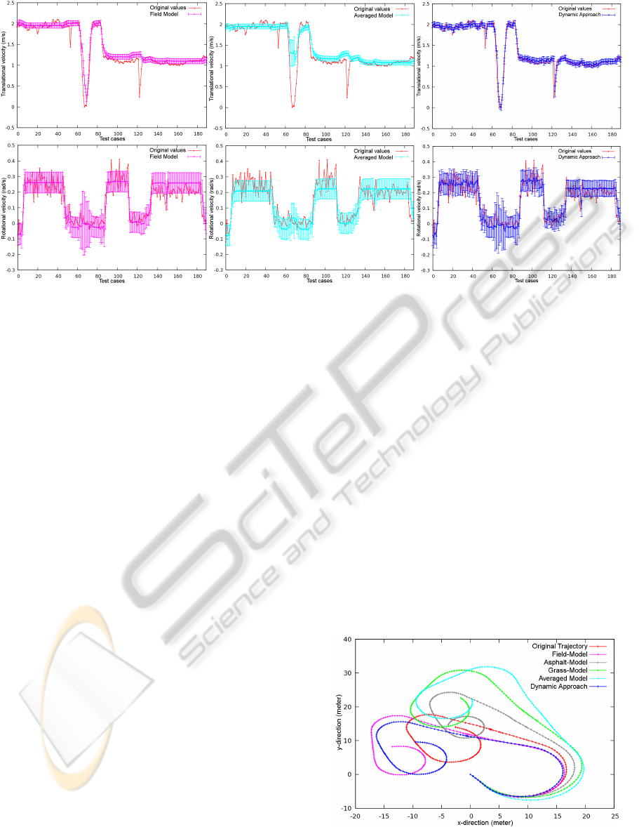
Figure 4: Estimation of the translational velocities (upper row), and of the rotational velocities (lower row) with error bars.

Even if the differences between the models are not signiﬁcant, they result in rather distinct trajectories.

5.1 Simple Approaches

We evaluated our approach on a test drive covering

three different terrains, starting on ﬁeld, continuing

with grass, and ending on asphalt. The test sequence

consists of 190 positions (about a 1 minute) almost

evenly partitioned on the three terrains. We compared

our dynamic approach to a ﬁeld model, an asphalt

model, a grass model and an averaged model. The

ﬁrst three models were trained only on the speciﬁc

terrain. The averaged model was trained on all three

terrains equally. All models used a total of 1500 train-

ing cases. The dynamic approach utilizes the three

terrain speciﬁc models.

We used the mean squared error (MSE) and the

standardized MSE to evaluate the quality of the re-

gression. The SMSE is the MSE divided by the vari-

ance of the test points, thus it does not depend on the

overall scaling of the values. The MSE is not applica-

ble to measure the quality of a trajectory because er-

rors at the beginning are propagated through the entire

trajectory inﬂuencing all proceeding positions. So we

introduced the mean segment distance error (MSDE).

First, we split the original trajectory and the predic-

tion in segments of ﬁxed size. Each pair of segments

is normalized to the same starting position and orien-

tation. The distance of the resulting end positions is

computed subsequently. The mean of all these dis-

tances constitutes the MSDE. We found a segment

size of 10 to be a reasonable size.

The estimation results of the translational (upper

row) and the rotational velocities (lower row) of the

ﬁeld model, the averaged model and of our dynamic

approach are shown in Figure 4. The ﬁeld model is

the best of the simple models. The averaged model

would be the model of choice if one wants to con-

sider different terrain conditions but does not want to

employ a dynamic approach.

The estimation of the translational velocities by

the averaged model shows little or no reaction to

any of the outliers. Averaging the effects of com-

mands over several terrains involves diminishing ef-

fects of certain command-terrain combinations, hence

causing inaccurate estimates. The ﬁeld model per-

forms best of the simple approaches, mainly because

it recognizes the slowdown around the 70th test case.

However, the other two outliers are not identiﬁed. The

estimates of the remaining test cases are similar to

the averaged model, yet the ﬁeld model is slightly

superior. Our dynamic approach outperforms both

Figure 5: Predicted trajectories. Starting the models’ pre-

dictions are exact but differ increasingly along the time line,

leading to unlike trajectories.

ICINCO 2010 - 7th International Conference on Informatics in Control, Automation and Robotics

Table 1: Prediction quality. The translational velocity unit

is m/s, the rotational velocity unit is rad/s, and the MSDE

unit is m.

Model MSE SMSE MSDE

v 0.02522 0.10588

Field

ω 0.00331 0.23605

0.42923

v 0.07032 0.29517

Asphalt

ω 0.00533 0.38034

0.56363

v 0.05161 0.21662

Grass

ω 0.00365 0.26041

0.51907

v 0.06203 0.26038

Averaged

ω 0.00377 0.26929

0.45478

v 0.01181 0.04956

Dynamic

ω 0.00279 0.19917

0.31407

previous models. In contrast, it recognizes all out-

liers, as the right terrain model is applied most of the

times. Additionally, the estimates of each test point

are pretty accurate.

The estimates of the rotational velocities give a

similar picture. The averaged model is somewhat off

at the beginning, underestimating the true values. The

ﬁeld model is much more accurate. The error bars

seem to be larger than in the upper row but it is due

to the scale of the data. However, our approach again

provides the best estimation, reacting even to minor

changes in the velocity values.

The velocities are translated into positions using

an UKF. The resulting trajectories of all models tested

are shown in Figure 5. The previous tendencies are

reﬂected in the quality of the trajectories. The aver-

aged model’s trajectory is rather inaccurate, followed

by the trajectory of the ﬁeld model which is outper-

formed by our dynamic approach. At the beginning

the predicted tracks are close, the differences start

during the ﬁrst turn and increase by the time. Even

though the distinction between the velocity estimates

are relatively small, the impact on the trajectories are

formidable. Especially the rotation values are crucial

Figure 6: Classiﬁcation results (upper image) and applied

models (lower image). The classiﬁcation matches the se-

quence of ﬁeld (red triangle), grass (green circles), and as-

phalt (grey squares) with high accuracy. Transitions are not

classiﬁable because the records contain data of two terrains.

Table 2: Classiﬁcation results and applied models. F = ﬁeld,

A = asphalt, G = grass.

Dynamic Approach Classiﬁcation Applied Model

Correct Terrain 96.06% 96.45%

p(y = F|x ∈ F) 100.00% 100.00%

p(y = A|x ∈ A) 93.75% 93.84%

p(y = G|x ∈ G) 94.44% 95.52%

to the trajectory quality.

We analyzed the quality of the GPR estimations

of the velocities with the MSE and the SMSE. Due

to the reasons mentioned above, the trajectories are

evaluated by the MSDE. The results are presented in

Table 1.

We also examined the classiﬁcation performance.

Figure 6 displays the results of the classiﬁcation af-

ter applying the BF, and the terrain models used for

the regression. The ﬁgures show that the classiﬁer

tends to categorize ﬁeld as grass vibrations and grass

records as asphalt. One problem is that the ﬁeld and

grass terrains are alike. At the low speed of approx-

imately 1 m/s the vibrations experienced on grass are

close to the ones recorded on asphalt. Nonetheless, al-

most all false classiﬁcations are compensated by the

BF.

Table 2 lists the classiﬁcation quality in terms of

correct classiﬁcations and applied models. Also, the

classiﬁcation rates are broken down into the classes

giving more insight.

5.2 Dynamic Approaches

In the previous section we compared our dynamic

approach to single terrain models, which by deﬁni-

tion cannot be optimal when the robot drives on sev-

eral different terrains. Therefore, we constructed an-

other dynamic approach similar to the one presented.

By doing so, we combined a support vector machine

(SVM) to perform the regression of the velocities,

and a k-nearest neighbor (k-NN) method for classi-

ﬁcation. We chose to combine a SVM and k-NN be-

cause of their low runtimes. The conducted experi-

ments showed the overall runtime of the GP approach

to be a serious issue.

We omitted the UKF from the system because the

SVM does not provide any uncertainty values. These

values are essential to the UKF in order to work prop-

erly. However, we kept the 2-step BF, even though

the k-NN method usually returns simple class labels

rather than class probabilities. We counted the votes

for each class and divided them by the total number

of neighbors k to provide class probabilities anyway.

We used the LibSVM library (Chang and Lin, 2001)

POSITION ESTIMATION OF MOBILE ROBOTS CONSIDERING CHARACTERISTIC TERRAIN PROPERTIES

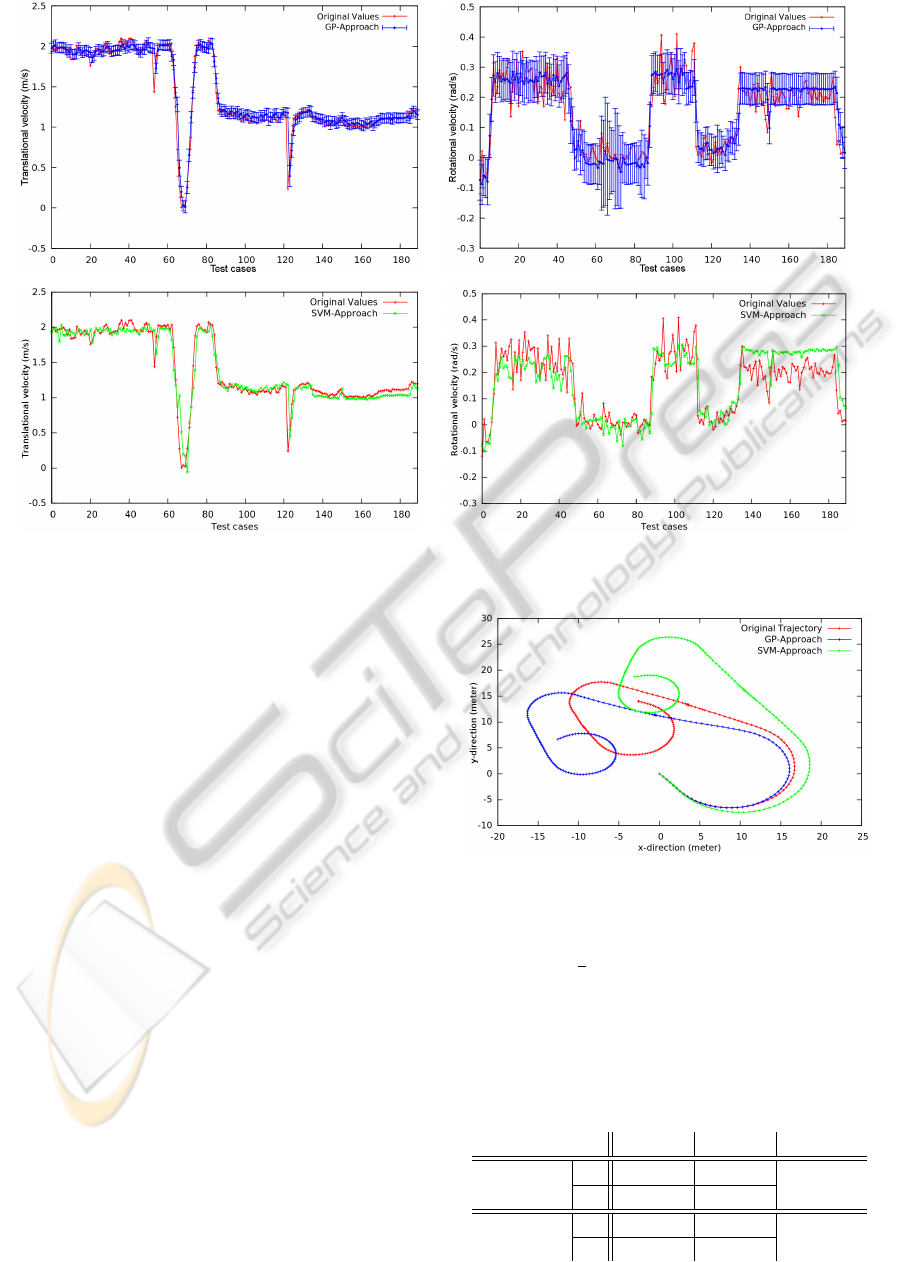
Figure 7: Comparison of the two dynamic approaches. Estimation of the translational velocities (left column), and of the

rotational velocities (right column) with error bars.

with a radial basis function (RBF) as SVM kernel and

found the OpenCV k-NN implementation with k = 8

neighbors to work best for vibrations.

To train the terrain models of the SVM we used

the same training data as we did for the GP models.

The training set of the classiﬁers are also unchanged.

Since this approach is able utilize several terrain

models for prediction, it should be more competitive

than the single terrain model approaches. To distin-

guish the two dynamic approaches, we will refer to

the GP based system as GP-Approach and to the SVM

and k-NN system as SVM-Approach.

The top row of Figure 7 shows the estimations of

the translational and rotational velocities by the GP-

Approach from the previous section. The prediction

results of the SVM-Approach are illustrated below.

Both dynamic approaches ﬁt the original translational

velocities fairly accurately and recognize all outliers.

The estimation differences between the two systems

are somewhat more apparent when we concentrate on

the rotational velocities. The SVM-Approach under-

estimates the ﬁrst part and overestimates the veloci-

ties towards the end. Its predictions are more agitated

in contrast to the averaging characteristic of the GP

estimations.

The observations are reﬂected in the error values

of Table 3. Even though the errors of the dynamic

approaches are very small - they are the smallest of

Figure 8: Predicted trajectories of the two dynamic ap-

proaches.

all tested models - the values of the SVM-Approach

are more than

higher. As we will see later, this is

partly due to the lower k-NN classiﬁcation quality.

The SVM’s underestimation of the rotational ve-

Table 3: Prediction quality of the two dynamic approaches.

The translational velocity unit is m/s, the rotational velocity

unit is rad/s, and the MSDE unit is m.

Model MSE SMSE MSDE

GP v 0.01181 0.04956

Approach ω 0.00279 0.19917

0.31407

SVM v 0.01923 0.08073

Approach ω 0.00464 0.33089

0.30336

ICINCO 2010 - 7th International Conference on Informatics in Control, Automation and Robotics

Table 4: Classiﬁcation results of the two dynamic ap-

proaches. F = ﬁeld, A = asphalt, G = grass.

Classiﬁcation SVM-Approach GP-Approach

Correct Terrain 70.00% 96.06%

p(y = F|x ∈ F) 71.43% 100.00%

p(y = A|x ∈ A) 93.75% 93.75%

p(y = G|x ∈ G) 55.55% 94.44%

Table 5: Applied models of the two dynamic approaches. F

= ﬁeld, A = asphalt, G = grass.

Applied Model SVM-Approach GP-Approach

Correct Terrain 75.26% 96.45%

p(y = F|x ∈ F) 71.70% 100.00%

p(y = A|x ∈ A) 91.04% 93.84%

p(y = G|x ∈ G) 62.86% 95.52%

locity corresponds to the assumption of a less sharper

turn. The green trajectory in Figure 8 shows exactly

this behavior. Furthermore, the higher estimated ro-

tational velocities at the end of the trajectory result in

tighter turns. Regardless of the rather different pre-

dictive trajectories, the trajectory qualities in Table 3

are almost the same.

With respect to the classiﬁcation task the GP clas-

siﬁer performs much better than the k-NN classi-

ﬁer. The sequence of classiﬁcations and applied

models are compared in Figure 9. While the GP-

Approach keeps the current terrain until enough ev-

idence is present that the terrain may have changed,

the SVM-Approach tends to change the terrain class

more quickly. This makes the system to apply the

wrong terrain model more often.

Table 4 and 5 point out that the k-NN classiﬁer

struggles to distinguish grass and ﬁeld records. Lead-

ing to a performance more than 25% worse than the

GP classiﬁcation. Evaluating the quality of the ap-

plied models, we can see a slight improvement by

about 5%, still staying way behind our approach.

Figure 9: Comparison of the two dynamic approaches.

Classiﬁcation results (upper image) and applied models

(lower image). Transitions are not classiﬁable because the

records contain data of two terrains.

As stated earlier the classiﬁcation quality is cru-

cial to the performance of the overall system, since

false classiﬁcations lead to the application of wrong

terrain models, resulting in worse velocity estima-

tions. However, the SVM-Approach, incorporating

SVM regression and k-NN classiﬁcation, is signiﬁ-

cantly faster than our GP-Approach.

6 CONCLUSIONS

In this paper we introduced a dynamic approach to

estimate positions of a mobile robot. Since the ter-

rain conditions are crucial to the robot’s implemen-

tation of velocity commands, we consider the terrain

for the prediction of future positions. We used GPs

for the regression of translational and rotational ve-

locities. An UKF transfers the velocity estimates into

positions and propagates the uncertainties of the posi-

tions over time. The vibration affecting the robot are

classiﬁed by a GPC model in order to separate differ-

ent terrains. A 2-step BF is used to compensate for

classiﬁcation errors and to model the terrain transi-

tions.

The prediction problem considered in this paper

has several difﬁcult properties: ﬁrst, with respect to

the classiﬁcation task, the visual ground truth is not

always accurate. Due to natural terrain types, which

in themselves can be vastly different, vibrations in-

duced by separate terrains may sometimes look alike

or even show characteristics of another terrain. In a

consequence, making it tricky to evaluate the the clas-

siﬁer’s performance. Second, ﬁnding a reasonable di-

versity of terrains is quite challenging, which aggra-

vates the task of determining the transition probabili-

ties from real data.

Nevertheless, our approach proved to be more

effective than simple approaches utilizing a single

model for all terrains. Furthermore, our GP-Approach

is competitive with other dynamic approaches using

different machine learning techniques. The dynamic

systems, our GP-Approach and the slightly struc-

turally altered SVM-Approach, are both better than

all simple models, proving the basic idea of our ap-

proach to be well suited to solve such prediction prob-

lems.

Future work will be to reduce the run time. Due to

the use of GPs the entire systems suffers of a long run

time. Several sparse algorithms for GPs exist which

would help to improve this issue. Moreover, expand-

ing the current system by additional terrains as sand

or gravel would be desirable. Extending the classiﬁ-

cation records by the translational velocity could im-

prove classiﬁcation results, since it allows to learn the

POSITION ESTIMATION OF MOBILE ROBOTS CONSIDERING CHARACTERISTIC TERRAIN PROPERTIES

effects of different speeds on the vibrations.

REFERENCES

Agrawal, M. and Konolige, K. (2006). Real-time localiza-

tion in outdoor environments using stereo vision and

inexpensive GPS. In International Conference on Pat-

tern Recognition (ICPR), volume 3, pages 1063–1068.

Brooks, C. A., Iagnemma, K., and Dubowsky, S. (2005).

Vibration-based terrain analysis for mobile robots. In

IEEE International Conference on Robotics and Au-

tomation (ICRA), pages 3415–3420.

Burgard, W., Fox, D., Hennig, D., and Schmidt, T. (1996).

Estimating the absolute position of a mobile robot us-

ing position probability grids. In AAAI National Con-

ference on Artiﬁcial Intelligence, volume 2.

Chang, C.-C. and Lin, C.-J. (2001). LIBSVM: a library

for support vector machines. Software available at

http://www.csie.ntu.edu.tw/∼cjlin/libsvm.

Dahlkamp, H., Kaehler, A., Stavens, D., Thrun, S., and

Bradski, G. R. (2006). Self-supervised monocular

road detection in desert terrain. In Robotics: Science

and Systems.

Ferris, B., H

ahnel, D., and Fox, D. (2006). Gaussian pro-

cesses for signal strength-based location estimation.

In Robotics: Science and Systems.

Girard, A., Rasmussen, C. E., Quinonero-Candela, J., and

Murray-Smith, R. (2003). Gaussian process priors

with uncertain inputs - Application to multiple-step

ahead time series forecasting. In Advances in Neural

Information Processing Systems (NIPS), pages 529–

536.

Iagnemma, K. and Ward, C. C. (2009). Classiﬁcation-

based wheel slip detection and detector fusion for mo-

bile robots on outdoor terrain. Autonomous Robots,

26(1):33–46.

Kapoor, A., Grauman, K., Urtasun, R., and Darrell, T.

(2007). Active learning with gaussian processes for

object categorization. In IEEE International Confer-

ence on Computer Vision (ICCV), volume 11, pages

1–8.

Ko, J., Klein, D. J., Fox, D., and H

ahnel, D. (2007a). Gaus-

sian processes and reinforcement learning for identiﬁ-

cation and control of an autonomous blimp. In IEEE

International Conference on Robotics and Automation

(ICRA), pages 742–747.

Ko, J., Klein, D. J., Fox, D., and H

ahnel, D. (2007b). GP-

UKF: Unscented Kalman ﬁlters with gaussian process

prediction and observationmodels. In IEEE/RSJ In-

ternational Conference on Intelligent Robots and Sys-

tems (IROS), pages 1901–1907.

Li-Juan, L., Hong-Ye, S., and Jian, C. (2007). Generalized

predictive control with online least squares support

vector machines. In Acta Automatica Sinica (AAS),

volume 33, pages 1182–1188.

MacKay, D. J. C. (1998). Introduction to gaussian pro-

cesses. In Bishop, C. M., editor, Neural Networks

and Machine Learning, NATO ASI Series, pages 133–

166. Springer-Verlag.

Rasmussen, C. E. (2002). Combining laser range, color, and

texture cues for autonomous road following. In IEEE

International Conference on Robotics and Automation

(ICRA).

Rasmussen, C. E. and Williams, C. K. I. (2005). Gaussian

Processes for Machine Learning. The MIT Press.

Seyr, M., Jakubek, S., and Novak, G. (2005). Neural net-

work predictive trajectory tracking of an autonomous

two-wheeled mobile robot. In International Federa-

tion of Automatic Control (IFAC) World Congress.

Thrun, S., Fox, D., Burgard, W., and Dellaert, F. (2000).

Robust monte carlo localization for mobile robot. Ar-

tiﬁcial Intelligence, 128:99–141.

Urtasun, R. and Darrell, T. (2007). Discriminative gaussian

process latent variable models for classiﬁcation. In In-

ternational Conference on Machine Learning (ICML).

Ward, C. C. and Iagnemma, K. (2007). Model-based wheel

slip detection for outdoor mobile robots. In IEEE In-

ternational Conference on Robotics and Automation

(ICRA), pages 2724–2729.

Weiss, C., Fr

ohlich, H., and Zell, A. (2006). Vibration-

based terrain classiﬁcation using support vector ma-

chines. In IEEE/RSJ International Conference on

Intelligent Robots and Systems (IROS), pages 4429–

4434.

Williams, C. K. I. (2002). Gaussian processes. In The Hand-

book of Brain Theory and Neural Networks. The MIT

Press, 2 edition.

ICINCO 2010 - 7th International Conference on Informatics in Control, Automation and Robotics