
NAVIGATION AND FORMATION CONTROL EMPLOYING
COMPLEMENTARY VIRTUAL LEADERS FOR COMPLEX
MANEUVERS
Martin Saska, Vojtˇech Von´asek and Libor Pˇreuˇcil
Department of Cybernetics, Czech Technical University in Prague, Technick´a 2, Prague, Czech Republic
Keywords:
Autonomous mobile robots, Compact formations, Virtual leaders, Trajectory planning.
Abstract:
Complex maneuvers of formations of car-like autonomous vehicles are investigated in this paper. The proposed
algorithm provides a complete plan for the formation to solve desired tasks and actual control inputs for each
robot to ensure collision-free trajectories with respect to neighboring robots as well as dynamic obstacles.
The method is based on utilization of complementary virtual leaders whose control inputs are obtained in one
merged optimization process using receding horizon control methodologies. The functionality of the system,
which enables reverse driving and arbitrary rotations of formations of nonholonomic robots, is verified by
simulations of multi-robot tasks and by hardware experiments.
1 INTRODUCTION
In this paper, we present a novel approach for a non-
holonomic robots formation driving and a trajectory
planning to reach a target region. The method al-
lows arbitrary maneuvers, including reverse driving
and turning of the formation in limited environment
with static as well as dynamic obstacles. Such skills
are crucial for the control of autonomous ploughs dur-
ing cooperative airport snow shoveling (Saska et al.,
2008; Hess et al., 2009) being our target applications.
Tasks for which autonomous vehicles in formation
are used usually involve physical constraints imposed
by the vehicles (mobility constraints) or physical ob-
stacles (environment constraints) and constraints en-
forced by inter vehicle relations (shape of the forma-
tion). Thus, it is important for control methodolo-
gies to incorporate system’s constraints into the con-
trollers design while preserving overall system sta-
bility which makes the Receding Horizon Control
(RHC) especially appealing. Receding horizon con-
trol (also known as model predictivecontrol) is an op-
timization based control approach often used for sta-
bilizing linear and nonlinear dynamic systems (e.g.,
see (Alamir, 2006) and references reported therein).
For a detailed survey of RHC methods we refer to
(Mayne et al., 2000) and references reported therein.
The works applying RHC for formation driving con-
trol are presented in (Dunbar and Murray, 2006)
(Franco et al., 2008). These papers have utilized RHC
for the formationforming and/or followingpredefined
trajectory in a workspace without obstacles. We will
apply the Receding Horizon Control for the virtual
leaders trajectory planning to desired goal area and
for the followers stabilization in the formation.
Our contribution is a general approach that ac-
counts for a nonholonomic robots’ formation stabi-
lization and a trajectory planning (enforced by a sta-
bility constraint) to reach a target region, also con-
sidering the response to dynamic changes in the en-
vironment. We developed a new concept of RHC by
combining both, the trajectory planning to the desired
goal region and the immediate control of the forma-
tion, into one optimization process. Our method can
continuously respond to changes in environment of
the robots while the cohesion of the immediate con-
trol inputs with direction of the formation movement
in future is kept. Furthermore, we extended the com-
mon leader-follower concept with the idea of two vir-
tual leaders, one for the forward and one for the back-
ward movement. Such an approach is necessary for
the complicated maneuvers of the formation of car-
like robots. The proposed method provides a com-
plete plan together with decisions when and how often
to switch between the guidance of the virtual leaders.
141
Saska M., Von
´
asek V. and P
ˇ
reu
ˇ
cil L. (2010).
NAVIGATION AND FORMATION CONTROL EMPLOYING COMPLEMENTARY VIRTUAL LEADERS FOR COMPLEX MANEUVERS.
In Proceedings of the 7th International Conference on Informatics in Control, Automation and Robotics, pages 141-146
Copyright
c
SciTePress

2 PRELIMINARIES
Let ψ
L
(t) = {x
L
(t),y
L
(t),θ
L
(t)} denote the configu-
ration of a virtual leader R
L
at time t,
1
and ψ
i
(t) =
{x
i
(t),y
i
(t),θ
i
(t)}, with i ∈ {1, . ..,n
r
}, denote the
configuration for each of the n
r
followers R
i
at
time t. The Cartesian coordinates (x
j
(t),y
j
(t)), j ∈
{1,...,n
r
,L} for an arbitrary configuration ψ
j
(t) de-
fine the position ¯p
j
(t) of a robot R
j
and θ
j
(t) denotes
its heading. Let us assume that the environment of
the robots contains a finite number n
0
of compact ob-
stacles collected in a set of regions O
obs
. Let us also
define a target region S
F
as a circle with radius r
S
F
and
centerC
S
F
such that O
obs
∩S
F
=
/
0. Finally, we need to
define a circular detection boundary with radius r
s
and
a circular avoidance boundary with radius r
a
, where
r
s
> r
a
. Single robots should not respond to obsta-
cles detected outside the region with radius r
s
. On the
contrary, distance between the robots and obstacles
less than r
a
is considered as inadmissable. These con-
cepts are adopted from the concept of avoidance con-
trol (Leitmann, 1980) to be used in this paper for the
collision avoidance guaranties. Moreover, we need to
extend these zones for the virtual leaders depending
on size of the formation to ensure that the result of
the leader trajectory planning is feasible also for the
followers. We will denote the extended radiuses as
r
s,L
and r
a,L
.
2.1 Kinematic Model and Constraints
The kinematics for any robots R
j
, j ∈ {1,...,n
r
,L},
in the formation is described by the simple non-
holonomic kinematic model: ˙x
j
(t) = v
j
(t)cosθ
j
(t),
˙y
j
(t) = v
j
(t)sinθ
j
(t),
˙
θ
j
(t) = K
j
(t)v
j
(t), where ve-
locity v
j
(t) and curvature K
j
(t) represent control in-
puts ¯u
j
(t) = (v
j
(t),K
j
(t)) ∈ R
2
.
Let us define a time interval [t
0
,t
N+M
] con-
taining a finite sequence with N + M + 1 el-
ements of nondecreasing times T (t
0
,t
N+M
) =
{t
0
,t
1
,...,t
N−1
,t
N
,...,t
N+M−1
,t
N+M
}, such that
t
0
< t
1
< ... < t
N−1
< t
N
< ... < t
N+M−1
< t
N+M
.
2
Also, let us define a controller for a robot
R
j
starting from a configuration ψ
j
(t
0
) by
U
j
(t
0
,t
N+M
,T (·)) := { ¯u
j
(t
0
;t
1
− t
0
), ¯u
j
(t
1
;t
2
−
t
1
),..., ¯u
j
(t
N+M−1
;t
N+M
− t
N+M−1
)} which is char-
acterized as a sequence of constant control actions.
Each element ¯u
j
(t
k
; t
k+1
−t
k
), k ∈ {0,...,N+M−1},
1
Index L denotes the virtual leader which has assigned
the leadership at the moment while indexes L
1
and L
2
dis-
tinguish between particular virtual leaders only if it is nec-
essary.
2
The meaning of constants N and M will be explained
in Section 3.
of the finite sequence U
j
(t
0
,t
N+M
,T (·)) will be held
constant during the time interval [t
k
,t
k+1
) with length
t
k+1
− t
k
(not necessarily uniform).
By integrating the kinematic model in over a given
interval [t
0
,t
N+M
], and holding constant control in-
puts over each time interval [t
k
,t
k+1
) (from this point
we may refer to t
k
using its index k), we can derive
the following model for the transition points at which
control inputs change:
x
j
(k+1) =
x
j
(k) +
1
K
j
(k+1)
sin
θ
j
(k)+
K
j
(k+1)v
j
(k+1)∆t(k+ 1)
−
sin
θ
j
(k)
,ifK
j
(k+1) 6= 0;
x
j
(k) + v
j
(k+1)cos
θ
j
(k)
∆t(k + 1),
if K
j
(k+1) = 0
y
j
(k+1) =
y
j
(k) −
1
K
j
(k+1)
cos
θ
j
(k)+
K
j
(k+1)v
j
(k+1)∆t(k+ 1)
−
cos
θ
j
(k)
,ifK
j
(k+1) 6= 0;
y
j
(k) + v
j
(k+1)sin
θ
j
(k)
∆t(k + 1),
if K
j
(k+1) = 0
θ
j
(k+1) = θ
j
(k) + K
j
(k+1)v
j
(k+1)∆t(k+ 1),
(1)
where x
j
(k) and y
j
(k) are the rectangular coordinates
and θ
j
(k) the heading angle for the configuration
ψ
j
(k) at the transition point with index k, v
j
(k + 1)
and K
j
(k + 1) are control inputs at time index k + 1,
and ∆t(k + 1) is the sampling time. This model and
notation allows us to describe long trajectories exactly
using a minimal amount of information such as: i) the
initial configurationψ
j
(t
0
), ii) the sequence of switch-
ing times T (·), and iii) the sequence of controls ac-
tions U
j
(·).
In real applications, the control inputs are lim-
ited by vehicle mechanical capabilities (i.e., chas-
sis and engine). This constraints can be taken into
account for each robot R
j
, j ∈ {1,...,n
r
,L}, limit-
ing their control inputs by the following inequalities:
v
min, j
≤ v
j
(k) ≤ v
max, j
and |K
j
(k)| ≤ K
max, j
, where
v
max, j
is the maximal forward velocity of the j-th ve-
hicle, v
min, j
is the limit on the backward velocity and
K
max, j
is the maximal control curvature. These values
can be different for each robot R
j
.
2.2 Formation Driving using RHC
The presented approach relies on the well known
leader-follower method frequently used in applica-
tions of car like robots (Barfoot and Clark, 2004).
In the method, the followers R
i
, i ∈ {1,...,n
r
} track
the leader’s trajectory which is distributed within the
group. The followers are maintained in relative dis-
tance to the leader in curvilinear coordinates with two
axes p and q, where p traces the leader’s trajectory
and q is perpendicular to p as is demonstrated in Fig-
ure 1. The positive direction of p is defined from R
L
back to the origin of the movement and the positive

p = p = p
q
1
1
L
3
2
1
6
5
4
9
8
7
q
3
2
3
p
q
q 0=
2
Figure 1: Formation described by curvilinear coordinates p
and q.
direction of q is defined in the left half plane in direc-
tion of the forward movement.
The shape of the formation is then uniquely deter-
mined by the parameters p
i
(t) and q
i
(t), defined for
each follower i, which can vary during the mission.
To convert the state of the followers in curvilinear co-
ordinates to the state in rectangular coordinates, the
simple equations in (Barfoot and Clark, 2004) can be
applied.
The main idea of the receding horizon control is to
solve a moving finite horizon optimal control problem
for a system starting from current states or configura-
tion ψ(t
0
) over the time interval [t
0
,t
f
] under a set of
constraints on the system states and control inputs. In
this framework, the length t
f
− t
0
of the time interval
[t
0
,t
f
] is known as the control horizon. After a so-
lution from the optimization problem is obtained on
a control horizon, a portion of the computed control
actions is applied on the interval [t
0
,δt
n
+ t
0
], known
as the receding step, where δt
n
:= ∆tn.
3
This pro-
cess is then repeated on the interval [t
0
+ δt
n
,t
f
+ δt
n
]
as the finite horizon moves by time steps defined by
the sampling time δt
n
, yielding a state feedback con-
trol scheme strategy. Advantages of the receding time
horizon control scheme become evident in terms of
adaptation to unknown events and change of strategy
depending on new goals or new events such as appear-
ing obstacles in the environment.
3 METHOD DESCRIPTION
In this section, a concept of complementary virtual
leaders, which enables backward driving of forma-
tions, will be proposed. The basic idea of the classical
leader-follower concept (see Figure 1) is based on the
fact that the followers continue with forward move-
ment until the place where the leader changed the po-
larity of its velocity. Such a behavior could cause col-
lisions or unacceptable disordered motion leading to
3
Number of applied constant control inputs n is chosen
according to computational demands as was explained in
(Saska et al., 2009).
a breakage of the shape of formation. Natural con-
ception of the formation movement supposes that the
entire group keeps compact shape and so all mem-
bers should change the polarity of their velocity in the
same moment.
Such an approach requires an extension of the
standard method employing one leader to an approach
with two virtual leaders, one for the forward move-
ment and one for the backward movement. Their
leading role is switched always when the sign of the
leader’s velocity is changed. The suspended virtual
leader becomes temporarily a virtual follower. The
virtual follower traces the virtual leader similarly as
the other followers to be able to undertake its leading
duties at time of the next switching. Therefore, all
robots in our system will be considered as followers
and there is no physical leader. The virtual leaders
will be positioned at the axis of the formation, one in
front of the formation and one behind the formation.
In the presented approach, we propose to solve
collision free trajectory planning and optimal control
together for both virtual leaders in one optimization
step. This ensures integrity of the solution for the
separated plants. Beyond this, we extend the stan-
dard RHC method with one control horizon into an
approach utilizing two finite time intervals T
N
and T
M
.
The first time interval T
N
should provide immediate
control inputs for the formation regarding the local
environment. By applying this portion of the control
sequence, the group is be able to respond to changes
in workspace that can be dynamic or newly detected
static obstacles. The difference ∆t(k+1) = t
k+1
−t
k
is
kept constant (later denoted only ∆t) in this time inter-
valand should satisfy the requirementsof the classical
receding horizon control scheme.
The second interval T
M
takes into account infor-
mation about the global characteristics of the environ-
ment to navigate the formation to the goal and to au-
tomatically compose the entire maneuver containing
usually multiple switching between the virtual lead-
ers. Here, we should highlight that also the number
of switchings between the virtual leaders is designed
automatically via the optimization process. The tran-
sition points in this part can be distributed irregularly
to effectively cover the environment. During the op-
timization process, more points should be automat-
ically allocated in the regions where a complicated
maneuver of the formation is needed. This is enabled
due to the varying values of ∆t(k+ 1) = t
k+1
− t
k
that
will be for the compact description collected into the
vector T
∆
L,M
= {∆t(N + 1), ...,∆t(N + M)}.
To define the trajectory planning problem with
two time intervals in a compact form we need to
gather states ψ
L
(k),k ∈ {1,...,N} and ψ
L
(k),k ∈

{N + 1,...,N + M} into vectors Ψ
L,N
∈ R
3N
and
Ψ
L,M
∈ R
3M
. Similarly the control inputs ¯u
L
(k),k ∈
{1,...,N} and ¯u
L
(k),k ∈ {N + 1,...,N + M} can be
gathered into vectors U
L,N
∈ R
2N
and U
L,M
∈ R
2M
.
In the case of the direction of movement alterna-
tion, the formation has to travel into the distance
max
i={1...n
r
}
p
i
to place the second virtual leader on
the position of the first one. Such a movement cre-
ates an
appendix
in the entire trajectory that is fol-
lowed. The minimal length of this additional tra-
jectory is defined by the size of the formation and
only the curvature of the leading robot is not uniquely
determined. Therefore, we have to define a vector
K
App
collecting variables K
App
( j),∀ j ∈ {1,...,N +
M − 1} applied for the movement of the virtual lead-
ers in the appendixes. N + M − 1 is maximal pos-
sible number of switchings. Usually the number of
switchings is significantly lower and the unused val-
ues of K
App
(·) will not be considered in the evalu-
ation of the optimization vector. All variables de-
scribing the complete trajectory from the actual po-
sition of the first virtual leader until target region
can be then collected into the unique optimization
vector Ω
L
= [Ψ
L,N
,U
L,N
,Ψ
L,M
,U
L,M
,T
∆
L,M
,K
App
] ∈
R
6N+7M−1
.u The vector Ω
L
contains necessary infor-
mation for both leaders, but we have to decide, which
part of the vector will be assigned to which leader.
Firstly, let us define an ordered set of indexes of
samples where the polarity of velocity is changed as
I
sw
:= {i : v
L
(i)v
L
(i+1) < 0},∀i∈ {1,...,N+M−1},
where the values of v
L
(·) can be extracted from the
vector U
L,MN
= [U
L,N
,U
L,M
] ∈ R
2(N+M)
. Now, we
can propose to collect the control inputs used for
the first virtual leader as U
L
1
,MN
= [ ¯u
L
(1), ¯u
L
(2),
..., ¯u
L
(I
sw
(1)), ¯u
App
1
(1), ¯u
F
1
(1), ¯u
L
(I
sw
(2) + 1),
¯u
L
(I
sw
(2) + 2), . . ., ¯u
L
(I
sw
(3)), ¯u
App
1
(2), ¯u
F
1
(2), ...,
¯u
L
(I
sw
(2n
sw
1
− 2) + 1), ¯u
L
(I
sw
(2n
sw
1
− 2) + 2), ... ,
¯u
L
(I
sw
(2n
sw
1
− 1)), ¯u
App
1
(n
sw
2
), ¯u
F
1
(n
sw
2
)], if n
sw
1
=
n
sw
2
and U
L
1
,MN
= [ ¯u
L
(1), ¯u
L
(2), ..., ¯u
L
(I
sw
(1)),
¯u
App
1
(1), ¯u
F
1
(1), ¯u
L
(I
sw
(2) + 1), ¯u
L
(I
sw
(2) + 2),
..., ¯u
L
(I
sw
(3)), ¯u
App
1
(2), ¯u
F
1
(2), ..., ¯u
App
1
(n
sw
2
),
¯u
F
1
(n
sw
2
), ¯u
L
(I
sw
(2n
sw
1
− 2) + 1), ¯u
L
(I
sw
(2n
sw
1
−
2) + 2), . .. , ¯u
L
(N + M)], if n
sw
1
6= n
sw
2
. The
control inputs for the second virtual leader as
U
L
2
,MN
= [ ¯u
F
2
(1), ¯u
L
(I
sw
(1) + 1), ¯u
L
(I
sw
(1) + 2),
..., ¯u
L
(I
sw
(2)), ¯u
App
2
(1), ¯u
F
2
(2), ¯u
L
(I
sw
(3) + 1),
¯u
L
(I
sw
(3) + 2), ..., ¯u
L
(I
sw
(4)), ¯u
App
2
(2), ¯u
F
2
(3), ...,
¯u
App
2
(n
sw
1
− 1), ¯u
F
2
(n
sw
1
), ¯u
L
(I
sw
(2n
sw
2
− 1) + 1),
¯u
L
(I
sw
(2n
sw
2
−1)+ 2), ..., ¯u
L
(N+M)], if n
sw
1
= n
sw
2
and U
L
2
,MN
= [ ¯u
F
2
(1), ¯u
L
(I
sw
(1) + 1), ¯u
L
(I
sw
(1) +
2), ... , ¯u
L
(I
sw
(2)), ¯u
App
2
(1), ¯u
F
2
(2), ¯u
L
(I
sw
(3) +
1), ¯u
L
(I
sw
(3) + 2), ..., ¯u
L
(I
sw
(4)), ¯u
App
2
(2), ¯u
F
2
(3),
..., ¯u
L
(I
sw
(2n
sw
2
− 1) + 1), ¯u
L
(I
sw
(2n
sw
2
− 1) + 2),
..., ¯u
L
(I
sw
(2n
sw
2
)), ¯u
App
2
(n
sw
1
− 1), ¯u
F
2
(n
sw
1
)], if
S
u ( )1
L
u ( )2
L
App
1
u ( )1
F
1
u ( )1
u ( )5
L
ψ (1)
L
Ψ (2)
L
ψ (4)
L
ψ (5)
L
(a) Trajectory of the first vir-
tual leader.
u ( )3
L
u ( )4
L
ψ (2)
L
ψ (3)
L
ψ (4)
L
S
F
2
u (2)
F
2
u ( )1
App
2
u ( )1
(b) Trajectory of the second
virtual leader.
Figure 2: Trajectories with denoted control inputs and states
of the two virtual leaders. The solid black curves denote
trajectories where the virtual leader is leading the formation
while the gray curves denote trajectories where the virtual
leader is the virtual follower. The initial positions of the
leaders are depicted by gray shadows.
n
sw
1
6= n
sw
2
.
The value n
sw
1
(resp. n
sw
2
) is number of time in-
tervals in which the first (resp. the second) virtual
leader has the leadership. Control inputs ¯u
F
1
( j),∀ j ∈
{1,...,n
sw
2
} (resp. ¯u
F
2
( j),∀ j ∈ {1,...,n
sw
1
}) are ob-
tained by the formation driving method when the first
(resp. the second) virtual leader is the virtual follower.
The control inputs ¯u
App
1
( j),∀ j ∈ {1,...,n
sw
1
} (resp.
¯u
App
2
( j),∀ j ∈ {1, . ..,n
sw
2
− 1}) are applied for the
formation driving in the appendixes and are obtained
using K
App
and v
max,L
.
The vectors T
∆
L
1
,MN
(resp. T
∆
L
2
,MN
) will be com-
piled similar as the vector U
L
1
,MN
(resp. U
L
2
,MN
),
because the variables ¯u(·) and ∆t(·) are inseparably
joined. An example illustrating this approach is pre-
sented in Figure 2 where the parameters and outputs
of the optimization are: N = 0, M = 5, I
sw
∈ {2,4},
U
L
1
= [ ¯u
L
(1), ¯u
L
(2), ¯u
App
1
(1), ¯u
F
1
(1), ¯u
L
(5)], U
L
2
=
[ ¯u
F
2
(1), ¯u
L
(3), ¯u
L
(4), ¯u
App
2
(1), ¯u
F
2
(2)].
The trajectory planning and the static as well as
dynamic obstacle avoidance problem for both virtual
leaders can be transformed to the minimization of sin-
gle cost function subject to sets of equality and in-
equality constraints. Accordingly the leader-follower
concept, the trajectory computed as the result of this
minimization will be used as an input of the trajec-
tory tracking for the followers. Details of the descrip-
tion of both, the leader trajectory planning and the
trajectory tracking for followers, can be found in our
previous publication in (Saska et al., 2009), where a
method with one leader enabling only forward move-
ment is presented.
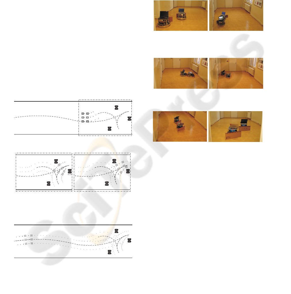
4 EXPERIMENTAL RESULTS
The results presented in this section have been ob-
tained using the introduced algorithm with parame-
ters: n = 2, N = 4, M = 8, and ∆t = 0.25s. In the
scenario of a road with obstacles in Figure 3 a for-
mation of 6 robots is aimed to reach the target region
in minimum time. In accordance with real applica-
tion, the maximum forward and backward velocities
of the virtual leader of the formation were set unsym-
metrically as v
min,L
= −v
max,L
/2. Putting the final re-
gion sufficiently far behind the formation, the solu-
tion of the formation to target zone problem is to turn
the formation and then continue forward to reach the
desired area. Such a maneuver, which contains two
switching between the virtual leaders, is denoted by
dashed curves in Figure 3(a). The solution of the task
keeps the formation outside the obstacles during the
whole maneuver. Beyond this, the ability to avoid
dynamic obstacles with collision course detected by
rear sensors of the robots during the reverse driving is
demonstrated in the simulation (see snapshots in Fig-
ure 3(b) and in Figure 3(c)). The complete history of
the turning can be seen in Figure 3(d).
Actual time: 0
(a) Initial position of the formation with complete plan for
both virtual leaders denoted by the dash curve.
Actual time: 6
(b) Detection of movement
of one obstacle and conse-
quential reaction of the fol-
lowers.
Actual time: 7.5
(c) The followers success-
fully passed by the obstacle
and they are going back to
their position in the forma-
tion.
Actual time: 15.75
(d) Accomplished task with denoted trajectories of the
robots.
Figure 3: Snapshots of turning 180 degrees in the environ-
ment with static as well as dynamic obstacles.
The presented simulations have shown only simple ex-
periments to demonstrate a basic behavior of the pre-
sented approach. More complicated scenarios prov-
ing the ability to avoid a damaged follower crossing
trajectories of neighbors, to utilize different shapes of
formations or to deal with local minima in a complex
environment cannot be offered due to space limitation
of this paper, but can be found in (Saska et al., 2009;
Saska et al., 2007).
t=0s
(a) Two indoor robots in
positions appropriate for
cooperative shoveling ma-
terials to the side.
t=17s
(b) Robots have changed
formation to a shape ap-
propriate for turning.
t=41s
(c) The second ”plough”
is overtaking the leader-
ship.
t=73s
(d) The leading duties are
going back to the first
robot.
t=98s
(e) The formation has fin-
ished the turning maneu-
ver.
t=115s
(f) Robots are again ready
for shoveling.
Figure 4: Formation turning at the end of a blind corridor.
The presented hardware experiment is a part of
airport snowshoveling project using formations of au-
tonomous ploughs, which has been reported in (Saska
et al., 2008; Hess et al., 2009). Here, we applied the
approach presented in this paper for turning the for-
mation of snow ploughs at the end of cleaning run-
way. The experiment has been performed on G2Bot
robotic platform equipped with SICK laser range
finder (not utilized in the experiment) and odometry.
In a simplified version of the experiments (see
snapshots in Figure 4, data from odometry in Figure 5
and a movie of the experiment in (MOVIE, 2010)),
two autonomous indoor robots are facing a blind cor-
ridor with an aim to turn at the end. The map of the
environment and positions of the vehicles are known
before the mission. During the experiment, positions
are updated using a dead reckoning because an exter-
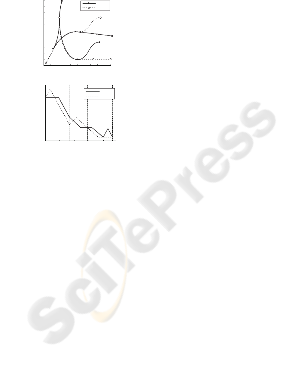
-5 -4.5 -4 -3.5 -3 -2.5 -2 -1.5 -1 -0.5 0
-0.2
0
0.2
0.4
0.6
0.8
1
1.2
1.4
1.6
1.8
t=115s
t=98s
t=115s
t=98s
t=0s
t=0s
t=17s
t=17s
t=41s
t=41s
t=73s
t=73s
2
Robot 1
Robot 2
x [m]
y [m]
(a)
0
25 50
75
100
-3.5
-3
-2.5
-2
-1.5
-1
-0.5
0
0.5
1
heading [rad]
time [s]
Robot 1
Robot 2
(b)
Figure 5: Data captured from odometry of both ploughs
with depicted times of snapshots in Figure 4.
nal positioning system is not necessary in such a short
term experiment. The actual position of robots and
their plans are shared via wireless communication.
The plan of robots is as follows: 1) build a compact
formation appropriate for turning, 2) turn 180 degrees
and 3) return back to the shoveling formation. Such
an approach is necessary in a case of largerformations
covering the whole runway and it can also better clar-
ify the method employing two virtual leaders. The
transitions between the different formations as well
as the turning maneuver are computed automatically
using the methods presented in this paper. Only the
positions of the vehicles within the formations (safety
distances, required overlapping of shovels etc.) are
given by experts.
5 CONCLUSIONS
In this paper, we have presented an RHC approach to
formation driving of car-like robots reaching a target
area in environments with obstacles. The proposed
approach is novel in the sense of utilized pair of com-
plementary virtual leaders necessary for guidance of
the formation during backward driving. This allows
us arbitrary maneuvers of formations including the U-
turn in bordered environment, which is necessary for
complete autonomous airport snow shoveling system.
The applicability of the presented approach has been
verified with simulations and hardware experiment.
ACKNOWLEDGEMENTS
This work is supported by the Czech Technical Uni-
versity under the grant SGS10/ 195/OHK3/ 2T/13
and by grants 2C06005 and MSM6840770038.
REFERENCES
Alamir, M. (2006). Stabilization of Nonlinear Systems Us-
ing Receding-Horizon Control Schemes, volume 339
of Lecture Notes in Control and Information Sciences.
Springer, Berlin / Heidelberg, Germany.
Barfoot, T. D. and Clark, C. M. (2004). Motion planning
for formations of mobile robots. Robotics and Au-
tonomous Systems, 46:65–78.
Dunbar, W. and Murray, R. (2006). Distributed receding
horizon control for multi-vehicle formation stabiliza-
tion. Automatica, 42(4):549–558.
Franco, E., Magni, L., Parisini, T., Polycarpou, M., and Rai-
mondo, D. (2008). Cooperative constrained control
of distributed agents with nonlinear dynamics and de-
layed information exchange: A stabilizing receding-
horizon approach. IEEE Transactions on Automatic
Control, 53(1):324–338.
Hess, M., Saska, M., and Schilling, K. (2009). Applica-
tion of coordinated multi vehicle formations for snow
shoveling on airports. Inteligent Service Robotics,
2(4):205 – 217.
Leitmann, G. (1980). Guaranteed avoidance strategies.
Journal of Optimization Theory and Applications,
32:569–576.
Mayne, D. Q., Rawlings, J. B., Rao, C. V., and Scokaert, P.
O. M. (2000). Constrained model predictive control:
Stability and optimality. Automatica, 36(6):789–814.
MOVIE (2010). Two indoor ploughs turning 360 degrees
[online]. [cit. 2010-1-13]. http://imr.felk.cvut.cz/ de-
mos/videos/files/shoveling.avi.
Saska, M., Ferenczi, I., Hess, M., and Schilling., K. (2007).
Path planning for formations using global optimiza-
tion with sparse grids. In In Proceedings of The 13th
IASTED International Conference on Robotics and
Applications (RA 2007)., Wuerzburg, Germany.
Saska, M., Hess, M., and Schilling, K. (2008). Effi-
cient airport snow shoveling by applying autonomous
multi-vehicle formations. In Proceedings of IEEE In-
ternational Conference on Robotics and Automation,
Pasadena, USA.
Saska, M., Mejia, J. S., Stipanovic, D. M., and Schilling, K.
(2009). Control and navigation of formations of car-
like robots on a receding horizon. In Proc of 3rd IEEE
Multi-conference on Systems and Control.
