SELECTION OF DIFFERENT PATHS FOR DOUBLY
NONHOLONOMIC MOBILE MANIPULATORS
Alicja Mazur and El˙zbieta Roszkowska
Institute of Computer Engineering, Control and Robotics,
Wrocław University of Technology, ul. Janiszewskiego 11/17, 50-372 Wrocław, Poland
Keywords:
Mobile manipulator, Nonholonomic constraints, Path following, Frenet parametrization.
Abstract:
This paper describes a problem of designing control laws preserving a motion along desired path for doubly
nonholonomic mobile manipulators. The doubly nonholonomic mobile manipulator is composed of a mobile
platform moving without slipping effect between wheels and the surface (i.e. nonholonomic platform) and an
onboard manipulator equipped with special nonholonomic gears, designed by Nakamura, Chung and Sørdalen.
A task for any nonholonomic subsystem (i.e. nonholonomic platform or nonholonomic manipulator) is to
follow a desired path – some geometric curve parameterized by curvilinear distance from selected point. A
description of the nonholonomic subsystem relative to the desired path using so-called Frenet parametrization
is a basis for formulating the path following problem and designing a kinematic control algorithm.
1 INTRODUCTION
A mobile manipulator is defined as a robotic system
which consists of a mobile platform, equipped with
non–deformable wheels, and a manipulator mounted
on the platform.
The problem with a path definition for the end-
effector of the mobile manipulator is that behavior
of the subsystems is unpredictable, because the same
path defined in global coordinates can be executed by
separate subsystems or by both of them. Sometimes,
it is important to move the platform and simultane-
ously unload a payload: such a task is defined rela-
tive to the base of the manipulator mounted on the
platform; definition relative to the end-effector is ill-
conditioned. In such situation the decomposition of
the task into tasks defined separately for both subsys-
tems is more natural and convenient (Mazur and Sza-
kiel, 2009).
In the paper we assume that a desired task can be
decomposed into two separate subtasks defined for
each subsystem independently: the end-effector has
to follow a desired geometric path described relative
to the base of manipulator (i.e. relative to the plat-
form) and the task of the platform is to follow a de-
sired curve lying on a plane. Such a formulation of
the task makes possible successive unloading of pay-
load transported by the mobile manipulator during the
control process.
X
P
P(s)
P
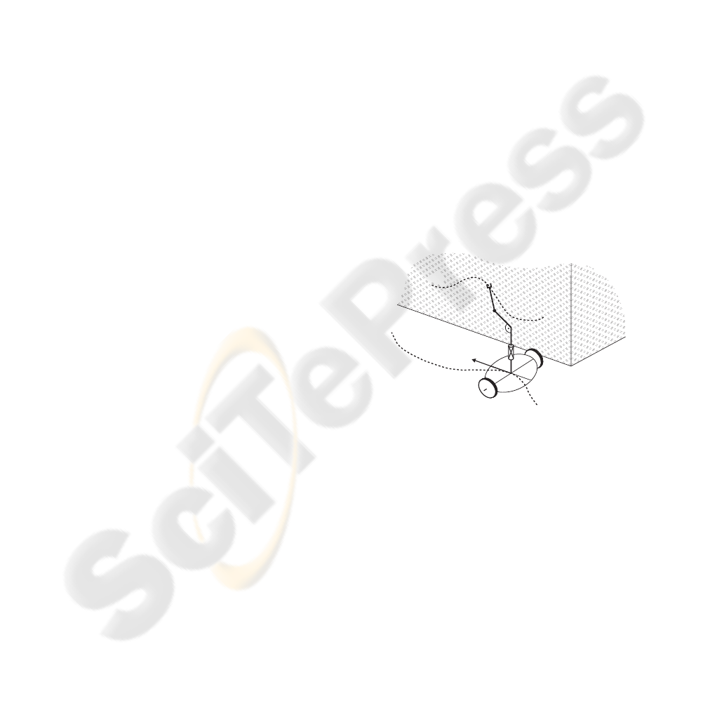
Figure 1: Decomposition of a task for doubly nonholo-
nomic mobile manipulator: P(s) – desired path for a non-
holonomic platform, Π(s) – desired path for a nonholo-
nomic manipulator.
Taking into account the type of components mo-
bility of mobile manipulators, there are 4 possible
configurations: type (h,h) – both the platform and
the manipulator holonomic, type (h,nh) – a holo-
nomic platform with a nonholonomic manipulator,
type (nh, h) – a nonholonomic platform with a holo-
nomic manipulator, and finally type (nh,nh) – both
the platform and the manipulator nonholonomic. The
notion doubly nonholonomic manipulator was intro-
duced in (Tcho´n et al., 2004) for the type (nh,nh).
15
Mazur A. and Roszkowska E. (2010).
SELECTION OF DIFFERENT PATHS FOR DOUBLY NONHOLONOMIC MOBILE MANIPULATORS.
In Proceedings of the 7th International Conference on Informatics in Control, Automation and Robotics, pages 15-21
Copyright
c
SciTePress
2 MATHEMATICAL MODELS OF
DOUBLY NONHOLONOMIC
MOBILE MANIPULATOR
In this paper we restrict our considerations to mobile
manipulators of (nh,nh) type, i.e. to doubly nonholo-
nomic objects. We will only discuss the constraints
occurring in the motion of both subsystems. Non-
holonomic constraints appearing in the motion of me-
chanical systems come from different sources. Very
often they come from an assumption that a motion of
the system can be treated as pure rolling of compo-
nents, without slippage effect. We have taken such as-
sumption in description of constrained motion of the
considered mobile manipulator.
2.1 Nonholonomic Constraints for
Wheeled Mobile Platform
Motion of the mobile platform can be described by
generalized coordinates q
m
∈ R
n
and generalized ve-
locities ˙q
m
∈R
n
. The wheeled mobile platform should
move without slippage of its wheels. It is equiva-
lent to an assumption that the momentary velocity at
the contact point between each wheel and the motion
plane is equal to zero. This assumption implies the
existence of l (l < n) independent nonholonomic con-
straints expressed in Pfaffian form
A(q
m
) ˙q
m
= 0, (1)
where A(q
m
) is a full rank matrix of (l×n) size. Since
due to (1) the platform velocity is in a null space of
A(q
m
), it is always possible to find a vector of special
auxiliary velocities η ∈ R
m
, m = n−l, such that
˙q
m
= G(q
m
)η, (2)
where G is an n ×m full rank matrix satisfying the
relationship AG = 0. We will call the equation (2) the
kinematics of the nonholonomic mobile platform.
2.2 Nonholonomic Constraints for
Manipulator
A rigid manipulator can be a holonomic or a non-
holonomic system – it depends on construction of its
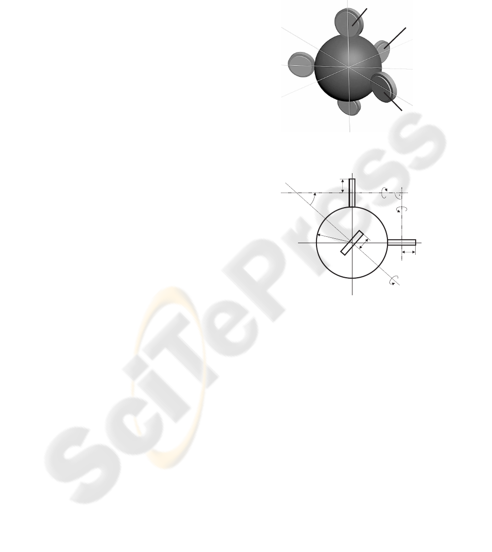
drives. In (Nakamura et al., 2001; Chung, 2004) the
authors have presented a new nonholonomic mechan-
ical gear, which could transmit velocities from the
inputs to many passive joints, see Figures 2-3. The
prototype of 4-link manipulator with such gears has
been developed in last 1990th years. Similar non-
holonomic 3-link manipulator is under construction at
Pozna´n University of Technology, Poland (Michałek
and Kozłowski, 2004). The nonholonomic constraints
in the gear appear by assumption on rolling contact
without slippage between balls of gear and wheels in
the robot joints.
OW
1
OW
2
IW
Figure 2: Schematic of the nonholonomic gear.
w
1,1
w
2,1
r
O
1
r
I
OW
2
OW
1
R
IW
r
O
2
a
O
a
I
q
1
Figure 3: Nonholonomic gear seen from above.
The basic components of the gear presented in
Figure 2 are a ball and three wheels – an input wheel
IW and two output wheels OW
1
and OW
2
. The veloc-
ity constraints of the ball are only due to point contact
with the wheels. The input wheel IW is mounted in
the first joint, the output wheels are mounted in the
next joint. The wheel IW rotates around the fixed
axis α
I
with an angular velocity u
2
, which plays the
role of a control input. The rotating input wheel IW
makes the ball rotate. The wheel OW
1
rotates around
an axis α
O
, which makes with the axis of the input
wheel a joint angle θ
1
. The angular velocity
˙
θ
1
= u
1
is the second control input for the manipulator with
nonholonomic gears.
Nonholonomic constraints (the kinematics) of n-
pendulum have the form
˙
θ
1
= u
1
, (3)
˙
θ
i
= a
i
sinθ
i−1
i−2
∏
j=1
cosθ
j
u
2
, i ∈{2, ... ,n}, (4)
with positive coefficients a
i
depending on gear ratios.
Hypothetical manipulator with 3 links and nonholo-
nomic gears has been presented in Figure 4.
θ
1
IW
ρ
θ
2
θ
3
Figure 4: Schematic of 3-link nonholonomic manipulator.
It is worth to emphasize that only two inputs u
1
and u
2
are able to control many joints of manipulator
equipped with gears designed by Nakamura, Chung
and Sørdalen.
3 DESCRIPTION OF
NONHOLONOMIC SYSTEM
RELATIVE TO A GIVEN PATH
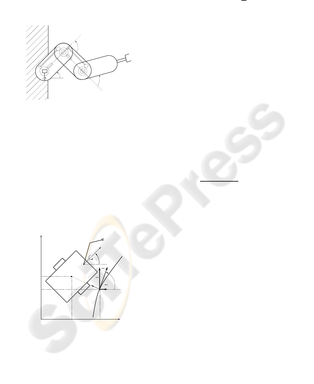
For nonholonomic systems whose workspace is pla-
nar, it is possible to describe state variables relative to
global inertial frame as well as to a given path (Mazur,
2004), see Figure 5.
r
X
0
0
Y
x
n
r
2
θ
2
M
θ
ω
v
M’
s
P
x
y
r
1
dr
ds
ds
dr
l
1
dr
ds
Figure 5: Illustration of path following problem for the non-
holonomic platform.
The path P is characterized by a curvature c(s),
which is the inversion of the radius of the circle tan-
gent to the path at a point characterized by the param-
eter s. Consider a moving point M and the associated
Frenet frame defined on the curve P by the normal
and tangent unit vectors x
n
and
dr
ds
. The point M is
the mass center of a mobile platform and M’ is the
orthogonal projection of the point M on the path P.
The point M’ exists and is uniquely defined if
the following conditions are satisfied (Fradkov et al.,
1999):
• The curvature c(s) is not bigger than 1/r
min
> 0.
• If the distance between the path P and the point M
is smaller than r
min
, there is a unique point on P
denoted by M’.
The coordinates of the point M relative to the Frenet
frame are (0, l) and relative to the basic frame X
0
Y
0
are
equal to (x,y), where l is the distance between M and
M’. A curvilinear abscissa of M’ is equal to s, where
s is a distance along the path from some arbitrarily
chosen point.
If we want to express the position of the point M
not in coordinates (x, y) relative to inertial frame, but
relative to the given path P, we should use some geo-
metric relationships, (Mazur, 2004),
˙
l = (−sinθ
r
cosθ
r
)
˙x
˙y
, (5)
˙s =
(cosθ
r
sinθ
r
)
1−c(s)l
˙x
˙y
, (6)
where ˙x and ˙y are defined by nonholonomic con-
straints for the system (wheeled mobile platform or
nonholonomic manipulator) and θ
r
is a desired orien-
tation at the point M’ on the path.
3.1 Path Following with Desired
Orientation
3.1.1 Nonholonomic Mobile Platform
Posture of the mobile platform is defined not only by
the position of the mass center, but by the orientation,
too. For this reason, it is necessary to define the ori-
entation tracking error equal to
˜
θ = θ−θ
r
. Moreover,
at the point M’ the desired orientation of the platform
fulfills a condition, (Samson, 1995),
˙
θ
r
= c(s)˙s. (7)
Then the coordinates
ξ = (l,
˜
θ,s)
T
(8)
i.e. the Frenet coordinates (l,s) and orientation track-
ing error
˜
θ, constitute path following errors for non-
holonomic mobile platform. It is worth to mention
that Frenet parametrization is valid only locally, near
the desired path.

As we mentioned earlier,out of Frenet coordinates
it is enough to consider only l and
˜
θ. Due to expres-
sions (5) and (7), Frenet variables for mobile platform
of (2,0) class described by nonholonomic constraints
˙x
˙y
˙
θ
=
cosθ 0
sinθ 0
0 1
v
ω
= G(q
m
)η (9)
can be defined as follows
(
˙
l = vsin
˜
θ,
˙
˜
θ =
˙
θ−
˙
θ
r
= ω−vcos
˜
θ
c(s)
1−c(s)l
= w,
(10)
where w is a new control input for the second equa-
tion.
For the system (10) we can use many control
laws, e.g. algorithm introduced in (Samson and Ait-
Abderrahim, 1991),
(
v = const
w = −k
2
lv
sin
˜
θ
˜
θ
−k
3
˜
θ, k
2
,k
3
> 0,
(11)
which is asymptotically stable. It can be shown using
the following Lyapunov-like function
V(l,
˜
θ) = k
2
l
2
2
+
˜
θ
2
2
(12)
and Barbalat lemma.
Path following with a desired orientation is very
important for mobile systems, especially for mobile
manipulators. It comes from the fact that it would
be impossible to unload a payload if the platform had
wrong orientation, i.e. it would be in a right place but
back-oriented.
3.1.2 Nonholonomic Manipulator
For a nonholonomic manipulator it is possible to fol-
low along the desired path with prescribed orienta-
tion. However, this issue has a drawback. Namely,
nonholonomic manipulator has only two control in-
puts, therefore it is impossible to have the mentioned
three parameters (l, s,
˜
θ) under control. In such a case
many authors decide to regulate only two tracking er-
rors (l,
˜
θ) to zero and they omit the differential equa-
tion for ˙s, because it does not matter at which point
s of the desired path the mobile platform enters the
desired curve P(s), see (Fradkov et al., 1999) for de-
tails. Such a case of the path following problem we
will call the asymptotic path following.
The Frenet parametrization can be evoked once
again in the problem of path following for the pla-
nar manipulator with nonholonomic gears moving on
the XZ surface.The role of the point M in Figure 5
plays a point at the end of a gripper. The orientation
of the end-effectorθ
m
is an rotation angle of the frame
associated with the gripper around –Y
b
axis, which is
located in the base of the manipulator. It means that
the orientation of the end-effector in the planar non-
holonomic n-pendulum is then equal to
θ
m
=
n
∑
i=1
θ
i
.
In the considered planar nonholonomic manipulator
lying in XZ-plane, relationships between velocity of
the working point M expressed in Cartesian and curvi-
linear coordinates have the form
˙
l
m
= (−sinθ
rm
cosθ
rm
)
˙x
˙z
, (13)
˙s =
(cosθ
rm
sinθ
rm
)
1−c(s)l
m
˙x
˙z
, (14)
where l
m
denotes distance between the point M and
the path Π(s), and θ
rm
is the orientation of the Frenet
frame in the point M’. Subscripts were introduced to
distinguish Frenet variables for both subsystems of
the (nh,nh) mobile manipulator.
Coordinates of the end-effector in the n-pendulum
relative to its base are equal to
x =
∑
n
i=1
l
i
cos
∑
i
j=1
θ
j
,
z =
∑
n
i=1
l
i
sin
∑
i
j=1
θ
j
.
(15)
Substituting time derivativesof variables (15), we ob-
tain the following equations
˙
l
m
=
n
∑
i=1
cos
θ
rm
−
i
∑
j=1
θ
j
!
l
i
i
∑
k=1
˙
θ
k
, (16)
˙
˜
θ
m
=
˙
θ
m
−c(s) ˙s =
n
∑
i=1
˙
θ
i
−
c(s)
1−c(s)l
m
·
·
n
∑
i=1
sin
θ
rm
−
i
∑
j=1
θ
j
!
l
i
i
∑
k=1
˙
θ
k
. (17)
Using the kinematics of the nonholonomic manipula-
tor given by (3)-(4), the equations (16) and (17) can
be expressed in the matrix form as follows
˙
ξ
m
=
˙
l
m
˙
˜
θ
m
= H(q
r
,ξ
m
)
˙
θ
1
.
.
.
˙
θ
n
=
= H(q
r
,ξ
m
)G
2
(q
r
)u = K
l
(q
r
,ξ
m
)u. (18)
Matrix K
l
(q
r
,ξ
m
) fulfills the regularity condition (i.e.
it is invertible) if some configurations, which imply
the matrix singularity, are excluded from a set of pos-
sibly achieved poses of the nonholonomic manipula-
tor.

For nonholonomic 3-pendulum matrix K
l
(q
r
,ξ
m
)
has the form
K
l
(q
r
,ξ
m
) =
K
l11
K
l12
K
l21
K
l22
,
with elements defined below
K
l11
=
3
∑
i=1
l
i
cos(θ
rm
−
i
∑
j=1
θ
i
),
K
l12
= a
2
s
1
3
∑
i=2
l
i
cos(θ
rm
−
i
∑
j=1
θ
i
) +
+a
3
s
2
c
1
l
3
cos(θ
rm
−
3
∑
j=1
θ
i
),
K
l21
= 1−
c(s)
1−c(s)l
m
3
∑
i=1
l
i
sin(θ
rm
−
i
∑
j=1
θ
i
),
K
l22
= a
2
s
1
[1−
c(s)
1−c(s)l
m
3
∑
i=2
l
i
sin(θ
rm
−
i
∑
j=1
θ
i
)]
+a
3
s
2
c
1
[1−
c(s)
1−c(s)l
m
l
3
sin(θ
rm
−
3
∑
j=1
θ
i
)].
Note that Frenet transformation is valid only locally,
i.e. l
m
(0) < r
min
, where r
min
is an inversion of max-
imal curvature c
max
of the manipulator path Π(s),
therefore nominators of all fractions are well defined.
In turn, the nonholonomic planar 3-pendulum cannot
achieve angles equal to θ
1
,θ
2
= 0,±π. Moreover,
singularities in K
l
matrix appear for sin(θ
rm
−θ
1
) =
sin(θ
rm
−θ
1
−θ
2
) = sin(θ
rm
−θ
1
−θ
2
−θ
3
) = 0.
For the regular matrix K
l
, the following control
signals guaranteeing a convergence of tracking errors
to zero for pure kinematic constraints can be proposed
u
r
= −K
−1
l
(q
r
,ξ
m
)Λξ
m
, Λ = Λ
T
> 0. (19)
It is easy to observe that the system (18) with closed-
loop of the feedback signal (19) has a form
˙
ξ
m
+ Λξ
m
= 0,
i.e. it is asymptotically stable.
3.2 Path Following without Desired
Orientation
The manipulator with gears designed by Nakamura,
Chung and Sørdalen has two control inputs. It means
that only two parameters can be regulated during the
path following process. If we mean that the orien-
tation of the end-effector of such manipulator is not
very important, it is possible to control other Frenet
parameters, e.g. l
m
– distance error from the desired
path and curvilinear length s of the path.
In such a case the following differential equations
˙
l
m
=
n
∑
i=1
cos
θ
rm
−
i
∑
j=1
θ
j
!
l
i
i
∑
k=1
˙
θ
k
,
˙s =
1
1−c(s)l
m
·
n
∑
i=1
sin
θ
rm
−
i
∑
j=1
θ
j
!
l
i
i
∑
k=1
˙
θ
k
have to be considered. Similarly to (16) and (17), us-
ing the kinematics of the nonholonomic manipulator
(3)–(4), these equations can be expressed in the ma-
trix form as follows
˙
l
m
˙s
= H(q
r
,ξ
m
)
˙
θ
1
.
.
.
˙
θ
n
= H(q
r
,ξ
m
)G
2
(q
r
)u
= K
s
(q
r
,ξ
m
)u. (20)
Matrix K
s
(q
r
,ξ
m
) fulfills the regularity condition (i.e.
it is invertible) if some configurations, which imply
the matrix singularity, are excluded from a set of pos-
sibly achieved poses of the nonholonomic manipula-
tor.
For nonholonomic 3-pendulum matrix K
s
(q
r
,ξ
m
)
has the form
K
s
(q
r
,ξ
m
) =
K
s11
K
s12
K
s21
K
s22
,
with elements defined below
K
s11
=
3
∑
i=1
l
i
cos(θ
rm
−
i
∑
j=1
θ
i
),
K
s12
= a
2
s
1
3
∑
i=2
l
i
cos(θ
rm
−
i
∑
j=1
θ
i
) +
+a
3
s
2
c
1
l
3
cos(θ
rm
−
3
∑
j=1
θ
i
),
K
s21
=
c(s)
1−c(s)l
m
3
∑
i=1
l
i
sin(θ
rm
−
i
∑
j=1
θ
i
),
K
s22
=
a
2
s
1
c(s)
1−c(s)l
m
3
∑
i=2
l
i
sin(θ
rm
−
i
∑
j=1
θ
i
)
+
a
3
s
2
c
1
c(s)
1−c(s)l
m
l
3
sin(θ
rm
−
3
∑
j=1
θ
i
).
Singular configurationsof nonholonomic3-pendulum
for the matrix K
s
are equal to configurations
sin(θ
1
) = sin(θ
1
−θ
2
) = sin(θ
1
−θ
2
−θ
3
) = 0.
If the following control law is applied
u
r
= −K
−1
s
(q
r
,ξ
m
)v, (21)
where v ∈ R
2
is a new input to the system (20), then
we obtain the decoupled and linearized control system
of the form
˙
l
m
˙s
=
v
1
v
2
. (22)
Now it is possible to control each variable separately.
For instance, if we want to move along the desired
path, not only to converge to this path, it seems to be
a good idea to preserve ˙s 6= 0. Possible choice of the
control algorithm for the decoupled system (22) is
v
1
= −Λl
m
, v
2
= const, Λ > 0.
Such control algorithm guarantees the motion along
the geometrical curve with constant velocity and, si-
multaneously, the convergence of the distance track-
ing error l
m
to 0.
4 SIMULATIONS
As an object of a simulation study we have chosen a
planar vertical 3-pendulum with nonholonomic gears
mounted on a unicycle.
The desired path for the manipulator (a circle ) was
selected as
Π
1
(s) = 0.25cos4s+ 1 [m],
Π
2
(s) = −0.25sin4s+ 0.6 [m],
and the desired path for the mobile platform was a
straight line
P(s) : x(s) =
√
2
2
s [m], y(s) =
√
2
2
[m].
The initial configuration of the manipulator was equal
to (θ
1
,θ
2
,θ
3
)(0)= (0,0.6732, −π/3) and initial pos-
ture of the platform was selected as (x,y,θ)(0) =
(0,2, 3π/4).
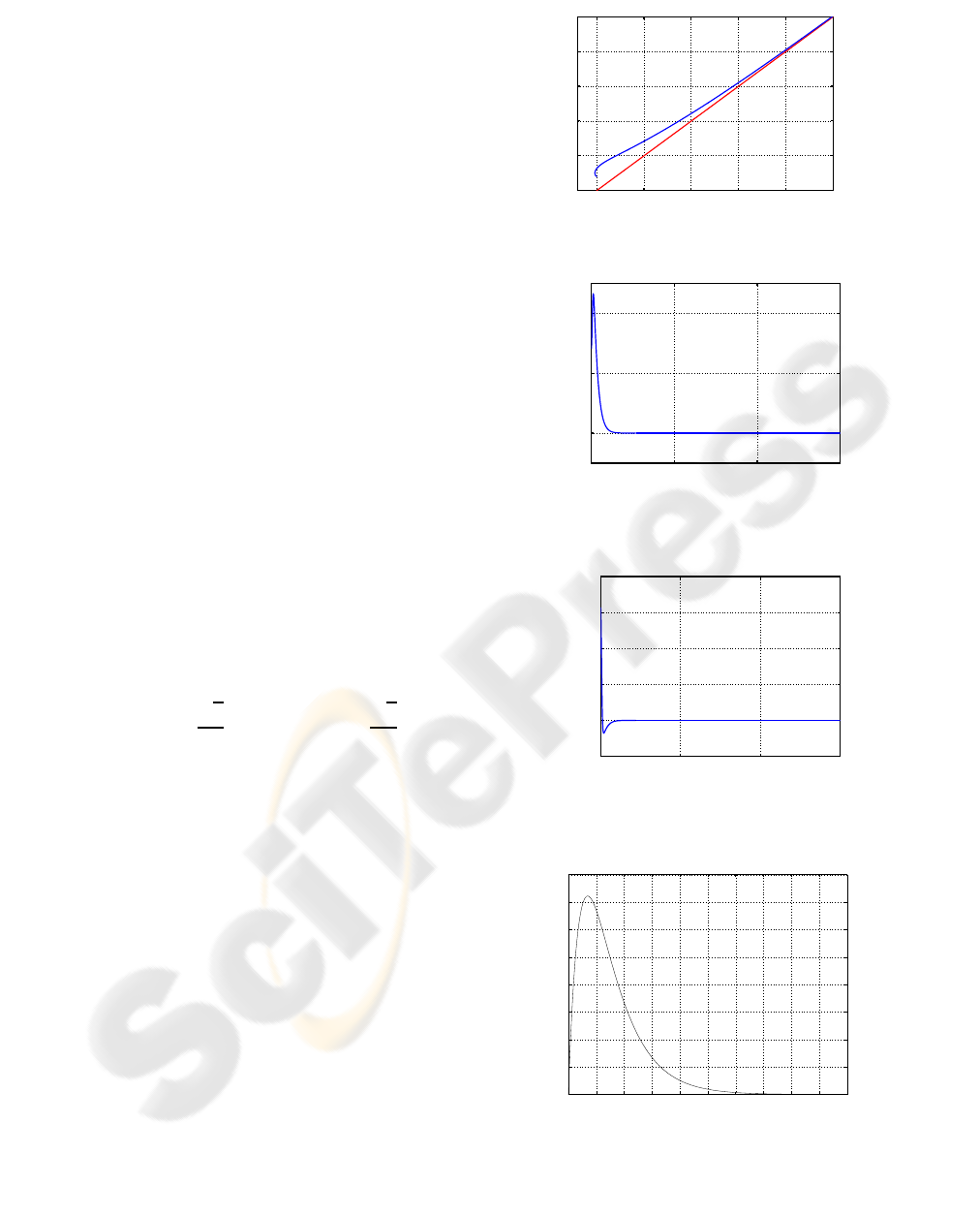
Tracking of the desired path for the mobile plat-
form has been presented in Figures 6–8. Parameters
of the Samson & Ait-Abderrahim algorithm were se-
lected as v = 1, k
2
= 0.1 and k
3
= 1.
Tracking of the desired path with prescribed orien-
tation for the nonholonomic manipulator 3R has been
presented in Figures 9–11.
Tracking of the desired path without preserved orien-
tation for the same manipulator has been presented in
Figures 12–13.
5 CONCLUSIONS
In the paper the problem of defining the path for dou-
bly nonholonomic mobile manipulators has been con-
sidered. We have proposed a new approach to the path
0 5 10 15 20 25
0
5
10
15
20
25
x [m]
y [m]
Figure 6: Path tracking for the mobile platform – XY plot.
0 200 400 600
0
1
2
time [s]
l [m]
Figure 7: Path tracking for the mobile platform – distance
error l.
0 200 400 600
−0.5
0
0.5
1
1.5
2
time [s]
θ−θ
r
[rad]
Figure 8: Path tracking for the mobile platform – orientation
error
˜
θ.
0 1 2 3 4 5 6 7 8 9 10
0
0.002
0.004
0.006
0.008
0.01
0.012
0.014
0.016
TIME [s]
Figure 9: Path tracking for the 3-pendulum: an error of x
coordinate.
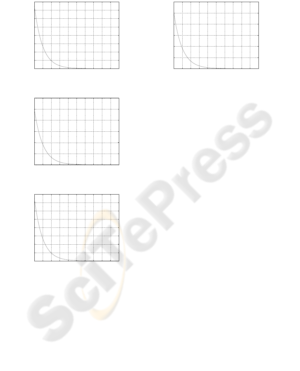
0 1 2 3 4 5 6 7 8 9 10
0
0.02
0.04
0.06
0.08
0.1
0.12
0.14
0.16
TIME [s]
Figure 10: Path tracking for the 3-pendulum: an error of z
coordinate.
0 1 2 3 4 5 6 7 8 9 10
0
0.02
0.04
0.06
0.08
0.1
0.12
TIME [s]
Figure 11: Path tracking for the 3-pendulum: an error of
orientation
˜
θ.
0 1 2 3 4 5 6 7 8 9 10
0
0.02
0.04
0.06
0.08
0.1
0.12
0.14
0.16
TIME [s]
Figure 12: Path tracking for the 3-pendulum – XZ plot.
as a geometric curve defined with the orientation or
not. Path following problem with prescibed orienta-
tion is very important for mobile systems, especially
for mobile manipulators – it results from the fact that
it is impossible to realize a task, namely unload a pay-
load if the platform has wrong orientation during the
regulation process.
In turn, for nonholonomic manipulator the desired
path need not be defined with orientation. In such a
case a new approach to the path following problem
has been presented in the paper. A new control algo-
rithm, guaranteeing not only asymptotic convergence
to the desired path but simultaneously the motion
0 1 2 3 4 5 6 7 8 9 10
0
0.02
0.04
0.06
0.08
0.1
0.12
TIME [s]
Figure 13: Path tracking for the 3-pendulum: a distance
error l
m
.
along the path with nonzero velocity, has been intro-
duced. It is possible to define another kinematic con-
trol algorithms with specific properties using Frenet
parametrization.
REFERENCES
Chung, W. (2004). Design of the nonholonomic manipula-
tor. Springer Tracts in Advanced Robotics, 13:17–29.
Fradkov, A., Miroshnik, I., and Nikiforov, V. (1999). Non-
linear and Adaptive Control of Complex Systems.
Kluwer Academic Publishers, Dordrecht.
Mazur, A. (2004). Hybrid adaptive control laws solv-
ing a path following problem for nonholonomic mo-
bile manipulators. International Journal of Control,
77(15):1297–1306.
Mazur, A. and Szakiel, D. (2009). On path following con-
trol of nonholonomic mobile manipulators. Interna-
tional Journal of Applied Mathematics and Computer
Science, 19(4):561–574.
Michałek, M. and Kozłowski, K. (2004). Tracking con-
troller with vector field orientation for 3-d nonholo-
nomic manipulator. In Proceedings of 4th int. Work-
shop on Robot Motion and Control, pages 181–191,
Puszczykowo, Poland.
Nakamura, Y., Chung, W., and Sørdalen, O. J. (2001).
Design and control of the nonholonomic manipula-
tor. IEEE Transactions on Robotics and Automation,
17(1):48–59.
Samson, C. (1995). Control of chained systems - ap-
plication to path following and time-varying point-
stabilization of mobile robots. IEEE Transactions on
Automatic Control, 40(1):147–158.
Samson, C. and Ait-Abderrahim, K. (1991). Feedback
control of a nonholonomic wheeled cart in cartesian
space. In Proc. of the IEEE Int. Conf. on Robotics and
Automation, pages 1136–1141, Sacramento.
Tcho´n, K., Jakubiak, J., and Zadarnowska, K. (2004).
Doubly nonholonomic mobile manipulators. In Pro-
ceedings of the IEEE International Conference on
Robotics and Automation, pages 4590–4595, New Or-
leans.
