
A PRACTICAL METHOD FOR SELF-ADAPTING GAUSSIAN
EXPECTATION MAXIMIZATION
Nicola Greggio
,‡
, Alexandre Bernardino
‡
and Jos
´
e Santos-Victor
‡
ARTS Lab - Scuola Superiore S. Anna, Polo S. Anna Valdera, Viale R. Piaggio, 34, 56025 Pontedera, Italy
‡
Instituto de Sistemas e Rob
´
otica, Instituto Superior T
´
ecnico, 1049-001 Lisboa, Portugal
Keywords:
Unsupervised learning, Self-adapting gaussian mixture, Expectation maximization, Machine learning, Clus-
tering.
Abstract:
Split-and-merge techniques have been demonstrated to be effective in overtaking the convergence problems in
classical EM. In this paper we follow a split-and-merge approach and we propose a new EM algorithm that
makes use of a on-line variable number of mixture Gaussians components. We introduce a measure of the
similarities to decide when to merge components. A set of adaptive thresholds keeps the number of mixture
components close to optimal values. For sake of computational burden, our algorithm starts with a low initial
number of Gaussians, adjusting it in runtime, if necessary. We show the effectivity of the method in a series
of simulated experiments. Additionally, we illustrate the convergence rates of of the proposed algorithms with
respect to the classical EM.
1 INTRODUCTION
UNSUPERVISED clustering classifies different data
into classes based on redundancy contained within the
data sample. The classes, also called clusters, are de-
tected automatically, i.e. without any input by an ex-
ternal agent. This method finds applications in many
fields, such as in image processing (e.g. segmentation
of different object from the background), sound anal-
ysis (e.g. word perceptions), segmentation of multi-
variate medical images, and many others. The tech-
niques for unsupervised learning range from Kohonen
maps, Growing Neural gas, k-means, to Independent
component analysis, Adaptive resonance theory, etc.
Particularly interesting is the Expectation Maximiza-
tion algorithm applied to Gaussian mixtures which al-
lows to model complex probability distribution func-
tions. Fitting a mixture model to the distribution of
the data is equivalent, in some applications, to the
identification of the clusters with the mixture compo-
nents (McLachlan and Peel, 2000).
Expectation-Maximization (EM) algorithm is the
standard approach for learning the parameters of the
mixture model (Dempster et al., 1977). It is demon-
strated that it always converges to a local optimum.
However, it also presents some drawbacks. For in-
stance, EM requires an a-priori selection of model
order, namely, the number of components (M) to be
incorporated into the model, and its results depend on
initialization. The more Gaussians there are within
the mixture, the higher will be the total log-likelihood,
and more precise the estimation. Unfortunately, in-
creasing the number of Gaussians will lead to overfit-
ting the data and it increases the computational bur-
den. Therefore, finding the best compromise between
precision, generalization and speed is a must. A com-
mon approach to address this compromise is trying
different configurations before determining the opti-
mal solution, e.g. by applying the algorithm for a dif-
ferent number of components, and selecting the best
model according to appropriate criteria.
1.1 Related Work
Different approaches can be used to select the best
number of components. These can be divided into
two main classes: off-line and on-line techniques.
The first ones evaluate the best model by execut-
ing independent runs of the EM algorithm for many
different initializations, and evaluating each estimate
with criteria that penalize complex models (e.g. the
Akaike Information Criterion (AIC) (Sakimoto et al.,
1986) and the Rissanen Minimum Description Length
(MDL) (Rissanen, 1989)). These, in order to be effec-
tive, have to be evaluated for every possible number of
models under comparison. Therefore, it is clear that,
36
Greggio N., Bernardino A. and Santos-Victor J. (2010).
A PRACTICAL METHOD FOR SELF-ADAPTING GAUSSIAN EXPECTATION MAXIMIZATION.
In Proceedings of the 7th International Conference on Informatics in Control, Automation and Robotics, pages 36-44
DOI: 10.5220/0002894600360044
Copyright
c
SciTePress

for having an sufficiently exhaustive search the com-
plexity goes with the number of tested models, and
the model parameters.
The second ones start with a fix set of models
and sequentially adjust their configuration (including
the number of components) based on different evalu-
ation criteria. Figueiredo and Jain proposed a method
that starts with a high number of mixture parame-
ters, merging them step by step until convergence
(Figueiredo and Jain, 2002). This method can be ap-
plied to any parametric mixture where the EM algo-
rithm can be used. Pernkopf and Bouchaffra proposed
a Genetic-Based EM Algorithm capable of learning
Gaussian mixture models (Pernkopf and Bouchaffra,
2005). They first selected the number of components
by means of the minimum description length (MDL)
criterion. A combination of genetic algorithms with
the EM has been explored.
Ueda et Al. proposed a split-and-merge EM al-
gorithm to alleviate the problem of local conver-
gence of the EM method (Ueda et al., 2000). Sub-
sequently, Zhang et Al. introduced another split-and-
merge technique (Zhang et al., 2003). The split-and-
merge equations show that the merge operation is a
well-posed problem, whereas the split operation is
ill-posed. Two methods for solving this problem are
developed through singular value decomposition and
Cholesky decomposition and then a new modified EM
algorithm is constructed. They demonstrated the va-
lidity of split-and-merge approach in model selection,
in terms of convergence properties. Moreover, the
merge an split criterion is efficient in reducing number
of model hypothesis, and it is often more efficient than
exhaustive, random or genetic algorithm approaches.
1.2 Our Contribution
In this paper, we propose an algorithm for comput-
ing the number of components as well as the param-
eters of the mixture model. Similarly to other split-
and-merge methods, our technique uses a local pa-
rameter search, that reuses the information acquired
on previous steps, being suitable to problems with
slowly changing distributions or to adapt the parame-
ters when new samples are added or removed. The
algorithm starts with a fixed number of Gaussians,
and automatically decides whether increasing or re-
ducing it. The key feature of our technique is the de-
cision of when add or merge a Gaussian. In order to
accomplish this at best we introduce a new concept,
the dissimilarity index between two Gaussian distri-
butions. Moreover, in order to evade local optimal
solutions we make use of self-adaptative thresholds
for deciding when Gaussians are split or merged. Our
algorithm starts with high thresholds levels, prevent-
ing large changes in the number of Gaussian compo-
nents at the beginning. It also starts with a low ini-
tial number of Gaussians, which can be increased dur-
ing computation, if necessary. The time evolution of
the threshold values allows periods of stability in the
number of components so that they can freely adapt
to the input data. After this period of stability these
thresholds become more sensitive, promoting the es-
cape from local optimum solutions by perturbing the
system configuration when necessary, until a stopping
criterion has reached. This makes our algorithm re-
sults less sensitive to initialization. The algorithm is
presented for Gaussian mixture models.
1.3 Outline
The paper is organized as follows. In sec. 2 we de-
scribe the notation and formulate the classical Expec-
tation Maximization algorithm. In sec. 3 we intro-
duce the proposed algorithm. Specifically, we de-
scribe the insertion of a new Gaussian in sec. 3.3,
its merging in sec. 3.4, the initializations in sec. 3.2,
and the decision thresholds update rules in sec. 3.5.
Furthermore, in sec. 4 we describe our experimen-
tal set-up for testing the validity of our new technique
and the results. Finally, in sec. 5 we conclude and
propose directions for future work.
2 EXPECTATION
MAXIMIZATION ALGORITHM
2.1 EM Algorithm: The Original
Formulation
A common usage of the EM algorithm is to iden-
tify the ”incomplete, or unobserved data” ¯y =
( ¯y
1
, ¯y
2
,... , ¯y
k
) given the couple ( ¯x, ¯y) - with ¯x defined
as ¯x = { ¯x
1
, ¯x
2
,. .. , ¯x
k
}, also called ”complete data”,
which has a probability density (or joint distribution)
p( ¯x, ¯y|
¯
ϑ) = p
¯
ϑ
( ¯x, ¯y) depending on the parameter
¯
ϑ.
We define E
0
(·) the expected value of a random vari-
able, computed with respect to the density p
¯
ϑ
( ¯x, ¯y).
We define Q(
¯
ϑ
(n)
,
¯
ϑ
(n−1)
) = E
0
L(
¯
ϑ), with L(
¯
ϑ)
being the log-likelihood of the observed data:
L(
¯
ϑ) = log p
¯
ϑ
( ¯x, ¯y)
(1)
The EM procedure repeats the two following steps
until convergence, iteratively:
A PRACTICAL METHOD FOR SELF-ADAPTING GAUSSIAN EXPECTATION MAXIMIZATION
37

• E-step: It computes the expectation of the joint
probability density:
Q(
¯
ϑ
(n)
,
¯
ϑ
(n−1)
) = E
0
[log p( ¯x, ¯y|
¯
ϑ
(n−1)
)]
(2)
• M-step: It evaluates the new parameters that max-
imize Q:
¯
ϑ
(n+1)
= argmax
¯
ϑ
Q(
¯
ϑ
n
,
¯
ϑ
(n−1)
)
(3)
The convergence to a local maxima is guaran-
teed. However, the obtained parameter estimates, and
therefore, the accuracy of the method greatly depend
on the initial parameters
ˆ
ϑ
0
.
2.2 EM Algorithm: Application to a
Gaussians Mixture
When applied to a Gaussian mixture density we as-
sume the following model:
p( ¯x) =
nc
∑
i=1
w
i
· p
i
( ¯x)
p
c
( ¯x) =
1
(2π)
d
2
|Σ
c
|
1
2
e
−
1
2
( ¯x−¯µ
c
)
T
|Σ
c
|
−1
( ¯x−¯µ
c
)
(4)
where p
c
(X ) is the component prior distribution for
the class c, and with d, ¯µ
c
and Σ
c
being the input
dimension, the mean and covariance matrix of the
Gaussians component c, and nc the total number of
components, respectively.
Consider that we have nc classes C
nc
, with p(¯x|C
c
)
and P(C
c
) = w
c
being the density and the a-priori
probability of the data of the class C
c
, respectively.
Then the E and M steps become, respectively:
E-step:
P(y
k
c
= 1|x
k
) = P(C
c
|x
k
) = E
0
(y
c
|x
k
)
=
p(x
k
|C
c
) · P(C
c
)
p(x
k
)
=
w
c
· p
c
(x
k
)
∑
nc
c=1
w
c
· p
c
(x
k
)
(5)
For simplicity of notation we refer to E
0
(y
c
|x
k
) as π
k
c
.
This is probability that the x
k
belongs to the class C
c
.
M-step:
¯µ
(n+1)
c
=
∑
k
i=1
π
k
c
¯x
i
∑
k
i=1
π
i
c
Σ
(n+1)
c
=
∑
k
i=1
π
k
c
( ¯x
i
− ¯µ
(n)
c
)( ¯x
i
− ¯µ
(n)
c
)
T
∑
k
i=1
π
i
c
(6)
Finally, a-priori probabilities of the classes, i.e. the
probability that the data belongs to the class c, are
reestimated as:
w
(n+1)
c
=
1
K
k
∑
i=1
π
i
c
, with c = {1, 2,. .. ,nc}
(7)
3 SAGEM: SELF-ADAPTING
GAUSSIAN EXPECTATION
MAXIMIZATION ALGORITHM
The key issue of our algorithm is looking whether one
or more Gaussians are not increasing their own likeli-
hood during optimization. In other words, if they are
not participating in the optimization process, they will
be split into two new Gaussians or merged. We will
introduce two new concepts related to the state of a
Gaussian component:
• The Area of a Gaussian, that measures how much
a Gaussian component covers the data space; This
actually correspond to the covariance matrix de-
terminant;
• Its age, that measures how long the component’s
own likelihood does not increase significantly (see
sec. 3.1);
Then, the merge and split processes are controlled by
the following adaptive thresholds:
• One adaptive threshold L
T H
for determining a sig-
nificant increase in likelihood (see sec. 3.5);
• One adaptive threshold A
T H
for triggering the
merge or split process based on the component’s
own age (see sec. 3.5);
• One adaptive threshold M
T H
for deciding to
merge two Gaussians based on their area and po-
sition (see sec. 3.4);
• One adaptive threshold S
T H
for deciding to split a
Gaussian based on its area (see sec. 3.3).
It is worth noticing that even though we consider
four thresholds to tune, all of them are adaptive, and
only require a coarse initialization. All these thresh-
olds cooperate in keeping the number of components
stable for a period after a split or merge operation (see
sec. 3.5).
These parameters will be fully detailed within the
next sections.
3.1 SAGEM Formulation
Our formulation can be summarized within four steps:
• Initializing the parameters;
• Adding a Gaussian;
• Merging two Gaussians;
• Updating decision thresholds.
Each Gaussian element i of the mixture is repre-
sented as follows:
¯
ϑ
i
= ρ(w
i
, ¯µ
i
,Σ
i
,ξ
i
,Λ
last
(i)
,Λ
curr
(i)
,a
i
)
(8)
ICINCO 2010 - 7th International Conference on Informatics in Control, Automation and Robotics
38

where w
i
is the a-priori probabilities of the class, ¯µ
i
is
its mean, Σ
i
is its the covariance matrix, ξ
i
its area,
Λ
last
(i)
and Λ
curr
(i)
are its last and its current log-
likelihood value, and a
i
its age. Here, we define two
new elements, the area and the age of the Gaussian,
which will be described later.
During each iteration, the algorithm keeps mem-
ory of the previous likelihood. Once the re-estimation
of the vector parameter
¯
ϑ has been computed in the
EM step, our algorithm evaluates the current log-
likelihood of each single Gaussian as:
Λ
curr
(i)
(ϑ) =
k−1
∑
j=0
log(w
i
· p
i
( ¯x
j
))
(9)
Then, for each Gaussian the difference between the
current and last log-likelihood value is compared with
a increment threshold, equal for all the Gaussians,
L
T H
. If the difference is smaller than the threshold
L
T H
, i.e. there is no significant increment, the algo-
rithm increases the age a
i
of the relative Gaussian. If
a
i
overcomes the age threshold A
T H
(i.e. the Gaus-
sian i does not increase its own likelihood for a prede-
termined number of times significally), the algorithm
decides whether to split this Gaussian or merging it
with existing ones.
Then, after a certain number of iterations the algo-
rithm will stop. The whole algorithm pseudocode is
shown in Fig. 3.1.
3.2 Split Threshold Initialization
At the beginning, S
T H
will be automatically initial-
ized to the area of the covariance of all the data set,
relative to the total mean. The other decision thresh-
olds will be initialized as follows:
M
T H−INIT
= 0
L
INIT
= k
L
T H
Age
INIT
= k
A
T H
(10)
with k
L
T H
and k
A
T H
(namely, the minimum
amount of likelihood difference between two itera-
tions and the number of iterations required for taking
into account the lack of a likelihood consistent vari-
ation) relatively low (i.e. both in the order of 10, or
20). Of course, higher values for k
L
T H
and smaller for
k
A
T H
give rise to a faster adaptation, however adding
instabilities.
3.3 Adding a Gaussian
If the covariance matrix area of the examined Gaus-
sian at each stage overcomes the maximum area
threshold S
T H
, then another Gaussian is added to the
mixture.
Algorithm 3.1. Pseudocode.
1: - Parameter initialization;
2: while (stopping criterion is not met) do
3: Λ
i
evaluation, for i = 0, 1,... ,c;
4: L(
¯
ϑ) evaluation (1);
5: re-estimate priors w
i
, for i = 0, 1,. ..,c;
6: recompute center ¯µ
(n+1)
i
and covariances Σ
(n+1)
i
, for
i = 0, 1,. ..,c (5);
7: - Evaluation whether changing the Gaussian
distribution structure -
8: for (i = 0 to c) do
9: if (a
i
> A
T H
) then
10: if ((Λ
curr
(i)
− Λ
last
(i)
) < L
T H
) then
11: a
i
+ = 1;
12: - General condition for changing satisfied;
now checking those for each Gaussians -
13: if (Σ
i
> S
T H
) then
14: if (c < maxNumGaussians) then
15: add Gaussian → split;
16: c+ = 1;
17: reset S
T H
to its initial value;
18: reset L
T H
to its initial value;
19: return;
20: end if
21: end if
22: for ( j = 0 to c) do
23: eval χ
i, j
(14)
24: if (χ
i, j
< M
T H
) then
25: merge Gaussian → merge;
26: c− = 1;
27: reset M
T H
to its initial value;
28: reset L
T H
to its initial value;
29: return;
30: end if
31: end for
32: S
T H
= S
T H
· (1 + α · ξ);
33: M
T H
= M
T H
· (1 + γ · χ
A,B
);
34: end if
35: end if
36: end for
37: end while
More precisely, the original Gaussian with param-
eters
¯
ϑ
old
will be split within other two ones. The new
means, A and B, will be:
¯µ
A
= ¯µ
old
+
1
2
(Σ
i= j
)
1
2
; ¯µ
B
= ¯µ
old
−
1
2
(Σ
i= j
)
1
2
i, j = {1,2, .. ., d}
(11)
where d is the input dimension.
The covariance matrixes will be updated as:
Σ
A
(i, j)
= Σ
old
(i, j)
; Σ
B
(i, j)
= Σ
old
(i, j)
i, j = {1,2, .. ., d}
(12)
The a-priori probabilities will be
w
A
=
1
2
w
old
; w
B
=
1
2
w
old
(13)
Finally, their ages, a
A
and a
B
, will be reset to zero.
A PRACTICAL METHOD FOR SELF-ADAPTING GAUSSIAN EXPECTATION MAXIMIZATION
39

3.4 Merging Two Gaussians
For each Gaussian B other than the given one A, the
algorithm evaluates a dissimilarity index. If that in-
dex is lower than the merge threshold M
T H
, Gaussian
B will be merged with Gaussian A. There are still no
exact methods for computing the overlap between two
Gaussians in arbitrary dimension. The existing meth-
ods use iterative procedures to approximate the de-
gree of overlap between two components (Sun et al.,
2007).
Here, we introduce a new dissimilarity index be-
tween Gaussian distributions, χ, that uses a closed
form expression, evaluated as follows:
χ
i, j
= kρ
i, j
+ δ
i, j
k
2
ρ
i, j
=
∑
i, j
kΣ
A
i, j
− µ
A
i
k · kΣ
B
i, j
− µ
B
i
k
ξ
i
· ξ
j
with i, j = {1,2, .. ., d}
(14)
where d is the input dimension, χ
i, j
is a new dis-
similarity index for mixture components, δ
i, j
is the
Euclidean distance between the two Gaussians i and
j. Another solution would have been to choose the
Mahalanobis distance (Mahalanobis, 1936) instead of
χ
i, j
. This takes into account both the mean an the co-
variance of the matrixes. Hoverer, the Mahalanobis
distance gives rise to zero if the two Gaussians have
the same mean, independently whether they cover the
same space (or, whether they have the same area ξ),
then rendering it not suitable for our purposes. Again,
we to avoid singularities, we use the area instead of
the covariance matrix determinant at the denomina-
tor of the correlation index ρ
i, j
. Finally, we defined
χ
i, j
as the square of the norm because this height-
ens values of kρ
i, j
+ δ
i, j
k > 1 while reducing those
kρ
i, j
+ δ
i, j
k < 1.
The new Gaussian (new) will have the following
mean and covariance:
µ
new
(i)
=
1
2
(µ
i
A
+ µ
i
B
); ρ
new
(i, j)
=
1
2
(ρ
A
i, j
+ ρ
B
i, j
)
with i, j = {1,2, .. ., d}
(15)
where d is the input dimension. The a-priori prob-
abilities for the remaining Gaussian will be updated
as:
c
new
= c
old
− 1; w
i
= w
i
+ w
old
/c
new
with i|
i6=old
= {1,2, .. ., c
new
}
(16)
Finally, like when adding a Gaussian, the age a
new
of the resultant Gaussian will be reset to zero.
3.5 Updating Decision Thresholds
The thresholds L
T H
, S
T H
, and ξ
T H
vary with the fol-
lowing rules:
L
T H
= L
T H
− λ · L
T H
= L
T H
· (1 − λ)
S
T H
= S
T H
+ α · (ξ − S
T H
) = S
T H
· (1 + α · ξ)
M
T H
= M
T H
+ γ · (χ
A,B
− M
T H
) = M
T H
· (1 + γ · χ
A,B
)
with ξ − S
T H
< 0, χ
A,B
− M
T H
> 0
(17)
with λ, α, and γ chosen arbitrarily low (we used λ =
0.04, α = 0.04, γ = 0.001). Following this rules L
T H
will decrease step by step, approaching the current
value of the global log-likelihood increment. This is
the same for S
T H
, which will become closer to the
area of some Gaussian, and for M
T H
that will in-
crease. This will allow the system to avoid some local
optima, by varying its configuration if a stationary sit-
uation occurs.
Finally, every time a Gaussian is added or merged,
these thresholds will be reset to their initial value.
3.6 Computational Complexity
Evaluation
Within this section we will use the following conven-
tion: ng is the number of the mixture Gaussian com-
ponents, k is the number of input vectors, d is the
number of input dimension, and it is the number of
iterations.
The computational burden of the EM algorithm is,
referring to the pseudocode in tab. 3.1 as follows:
• the original EM algorithm (steps 3 to 6) take O(k ·
d · ng) for 3 and 6, while step 4 and step 5 take
O(1) and O(k · ng);
• our algorithm takes O(ng) for evaluating all the
Gaussians (step 8 to 36) and another O(ng) in step
23 for evaluating the dissimilarity between each
Gaussian (14);
• our merge and split (step 15 and 25) operations
require O(d) and O(d · ng), respectively.
• the others take O(1).
Therefore, the original EM algorithm takes O(k · d ·
ng), while our algorithm adds O(d ·ng
2
) on the whole,
giving rise to O(k · d · ng) + O(d · ng
2
) = O(k · d · ng +
d · ng
2
) = (ng · d · (k + ng)). Considering that usually
d << k and ng << k this does not add a considerable
burden, while giving an important improvement to the
original computation in terms of self-adapting to the
data input configuration at best.
ICINCO 2010 - 7th International Conference on Informatics in Control, Automation and Robotics
40

4 EXPERIMENTAL VALIDATION
In order to evaluate the performance of our algorithm,
we tested it by classifying different input data ran-
domly generated by a known Gaussian mixture, and
subsequently saved to a file. This is in order to use
the same input data to our algorithm, SAGEM, and to
the original EM. Our algorithm starts with a low ini-
tial number of Gaussians, while the original EM starts
with the exact number of Gaussians, i.e. the mixture
configuration we generated the input data points from.
Moreover, in order to make a fair comparison, both
the algorithms started with the same input Gaussian
means (of course, since SAGEM has fewer Gaussian
components than EM these are a subset of those of
EM).
We refer to the EM with the exact number of
Gaussians that generated the input data as the best EM
algorithm applicable, i.e. the algorithm that uses the
best compromise between number of Gaussian com-
ponents and final likelihood. Therefore, we will use
its results as comparison for our algorithm.
4.1 Experimental Set-up
We made different trials, with mixtures containing 4,
8, 12, 14, and 16 Gaussians. Each of them contains
2000 points in two dimensions. We choose to show
the results for 2-dimensional input because they are
easier to show than multidimensional ones (for in-
stance, a 2-dimensional Gaussian is represented in
2D as an ellipse). As the ratio (# Gaussians)/(# data
points) increases, it become harder to reach a good so-
lution in the reasonable number of steps. Therefore,
we are interested in evaluating how SAGEM behaves
when the model complexity gradually increases.
We evaluated the performance of our algorithm
compared with the original EM principally based on
three main points:
• Final log-likelihood value;
• Final number of Gaussian components;
• Number of iterations needed for reaching stability.
Therefore, we used the following equations for
evaluating the error on the final Log-likelihod, and
the error on the predicted number of Gaussian com-
ponents as follows, respectively (the required number
of iterations can be extracted from the plots in Fig. 1,
directly.
Log − Lik
err
=
Log − Lik
(SAGEM)
Log − Lik
(EM)
NumGauss
err
= NumGauss
(SAGEM)
− NumGauss
(EM)
(18)
In table I the output of the different computations
are shown.
The results will be discussed within the next sec-
tion.
4.2 Discussion
The output of the two algorithms is shown in Fig.
1. The input data (green points) with the genera-
tion mixture (blue) and the evaluated one (red) are
represented in the same figure, while the resultant
log-likelihood (blue for the EM algorithm and red
for SAGEM) is shown. It is worth noticing that we
also represented the iterations at which a split or a
merge operation is performed, as vertical blue and
red lines, respectively. Here, it is possible to see how
just after a splitting or merging operation the final log-
likelihood has some spikes. When a merge operation
is performed the algorithm decreases the number of
Gaussian components, therefore decreasing the log-
likelihood momentarily abruptly. An example is at
iteration 92 of the 12-Gaussian plot. Besides, when
a new class is added by means of a splitting opera-
tion, it may happen that the final log-likelihood starts
increasing smoothly due to the new component’s con-
tribute (e.g. see the 8-Gaussian plot at iteration 22, or
the 14-Gaussian plot at iteration 50), or has a decreas-
ing spike (e.g. see the 8-Gaussian plot at iteration 34
or 53) If the components are reorganized by the EM
procedure in order to describe the data better, the log-
likelihood will start to increase smoothly.
Finally, Fig. 2.6 shows the 3D histogram repre-
sentation of a generated Gaussian mixture data and
the estimated one. Due to space limitations, we
choose to show only the one that gave rise to the
worst log-likelihood estimation plot, i.e. the one with
8 Gaussians.
In table I the results of the different computations
are shown. The table contains, for both SAGEM and
the EM algorithm:
• The starting number of Gaussian components;
• The final (i.e. detected, in the case of the SAGEM
approach) number of Gaussian components;
• The error on the final number of components.
• The final reached log-likelihood.
• The error on the final log-likelihood, as absolute
value.
Due to the formulation in (18), if Log − Lik
err
< 1
than SAGEM reached a final log-likelihood greater
than EM (both are negative), and vice versa. Simi-
larly, when NumGauss
err
< 0 it means that SAGEM
A PRACTICAL METHOD FOR SELF-ADAPTING GAUSSIAN EXPECTATION MAXIMIZATION
41
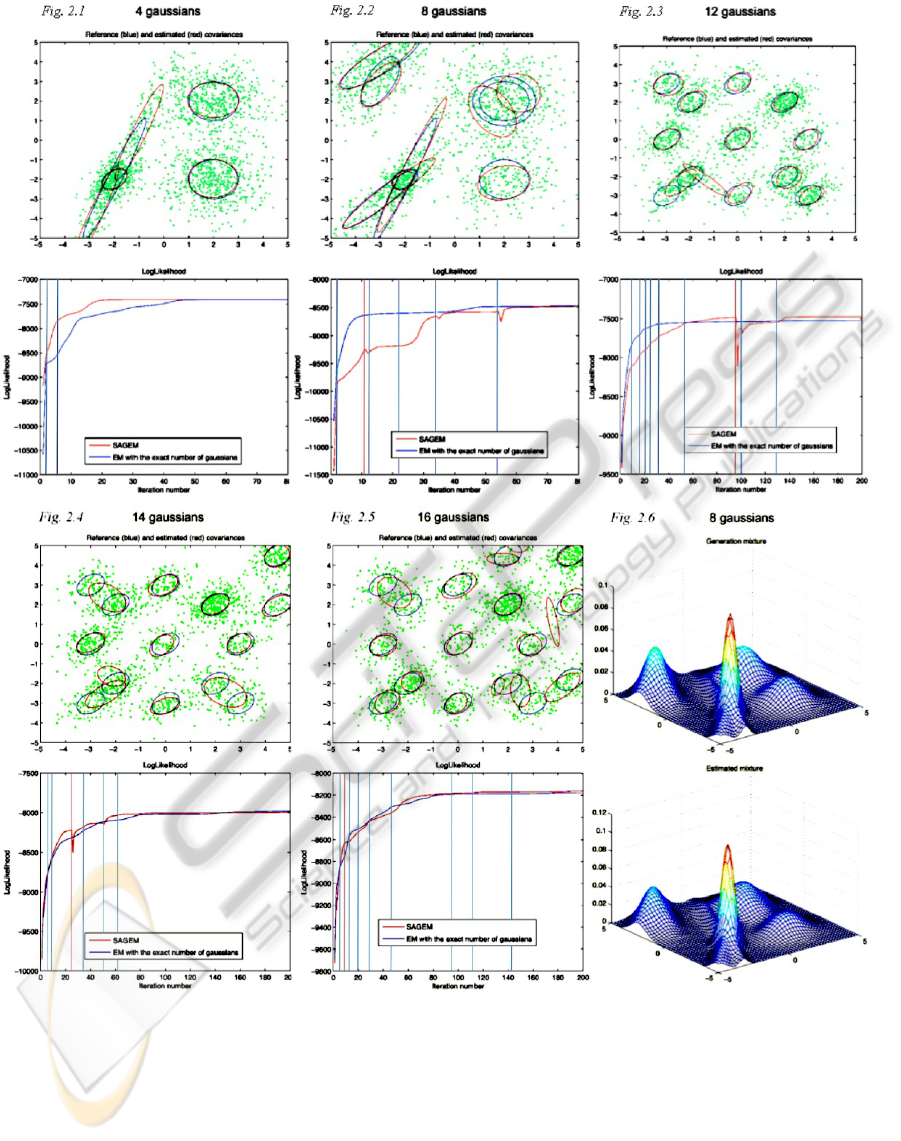
Figure 1: The 2D representation of the final SAGEM Gaussian mixture vs. the real one and the SAGEM and EM log-
likelihood output as function of the iterations number, for different input mixtures of data (4, 8, 12, 14, and 16 Gaussian
components). Moreover the 8-Gaussians case comparison between the generated and computed mixtures is shown.
used fewer Gaussians then real ones. These two com-
parisons are shown in plots 2(a), 2(b), and 2(c) re-
spectively.
We can see that the final SAGEM log-likelihood
is often better than the one obtained with the original
EM with the exact number of Gaussians, except for
the case of 8-Gaussians. There are three interesting
points:
• Within the 14-Gaussians case SAGEM reached
a higher log-likelihood than EM even with less
Gaussians components than required.
• Increasing the number of components, the points
representing each class will be fewer. This in-
ICINCO 2010 - 7th International Conference on Informatics in Control, Automation and Robotics
42
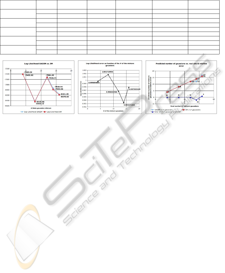
Table 1: Experimental results.
Number of effective Algorithm Starting number Arrival number Error on the number Final log-likelihood Error on the final
mixture Gaussians of Gaussians of Gaussians of Gaussians log-likelihood
4 SAGEM 2 4 0 -7402.82 -2.26
EM 4 4 / -7405.08 /
8 SAGEM 4 8 0 -8448.56 14.43
EM 8 8 / -8434.13 /
12 SAGEM 6 12 0 -7501.62 -28.36
EM 12 12 / -7526.74 /
14 SAGEM 8 12 -2 -7928.95 -53.71
EM 14 14 / -7982.66 /
16 SAGEM 10 17 +1 -8161.29 -17.13
EM 16 16 / -8178.42 /
Figure 2: The final log-likelihood of both SAGEM and EM as function of the number of input data Gaussian components (a),
the relative error (b), and the final reached number of Gaussians as function of the input ones (c).
creases the difficulty of clustering them into dis-
tinct classes. Nevertheless, SAGEM has been able
to detect a number of required Gaussians close to
the original one (12 vs. 14 and 17 vs. 16), and to
have a better final log-likelihood than EM.
• Regarding to the plots of the log-likelihood we
can see that both SAGEM and EM reach a sim-
ilar likelihood within the first 60-80 iterations,
even though EM is usually faster in increasing it.
Some spikes in the SAGEM plots occur, due to
the modification of the number of Gaussians. In
fact, when merging two mixture components the
log-likelihood momentarily decreases.
• Even though the 8-Gaussian case is the worst one
in terms of final likelihood, the histogram of the
final Gaussian mixture is very similar to the true
one.
5 CONCLUSIONS AND FUTURE
WORK
In this paper we proposed a new split-and-merge Ex-
pectation Maximization algorithm, called SAGEM.
The algorithm is specific for Gaussian mixtures.
SAGEM starts with a fixed number of Gaussians, and
automatically decides whether increasing or reducing
it. We introduced a new concept, a dissimilarity in-
dex between two Gaussian distributions. Moreover,
in order to evade local optimal solutions we make use
of self-adaptative thresholds for deciding when Gaus-
sians are split or merged. We tested it with different
Gaussian mixtures, comparing its results with those
of the EM original algorithm set with the model com-
plexity that matches those we generated the data from
(ideal case). We showed that our algorithm is capable
to evaluate a number of Gaussian components close
to the true one, and to provide a final mixture descrip-
tion with a log-likelihood comparable with the orig-
inal EM, sometimes even better. Finally, its conver-
gence occurs with the same number of iterations than
it does for the original EM (60-80 iterations).
5.1 Future Work
At the moment we tested our algorithm with synthetic
data. As future work, we will test SAGEM for the
purpose of image segmentation on real images cap-
tured in order to test it in real robotic applications,
where the computational burden must be kept low.
More specifically, being part of the RobotCub Euro-
pean Project, we will test it with the iCub robotics
platform.
A PRACTICAL METHOD FOR SELF-ADAPTING GAUSSIAN EXPECTATION MAXIMIZATION
43

ACKNOWLEDGEMENTS
This work was supported by the European Com-
mission, Project IST-004370 RobotCub and FP7-
231640 Handle, and by the Portuguese Government -
Fundac¸
˜
ao para a Ci
ˆ
encia e Tecnologia (ISR/IST
pluriannual funding) through the PIDDAC program
funds and through project BIO-LOOK, PTDC / EEA-
ACR / 71032 / 2006.
REFERENCES
Dempster, A., Laird, N., and Rubin, D. (1977). Maximum
likelihood estimation from incomplete data via the em
algorithm. J. Royal Statistic Soc., 30(B):1–38.
Figueiredo, A. and Jain, A. (2002). Unsupervised learn-
ing of finite mixture models. IEEE Trans. Patt. Anal.
Mach. Intell., 24(3).
Mahalanobis, P. C. (1936). On the generalized distance in
statistics. Proceedings of the National Institute of Sci-
ences of India, 2(1):39–45.
McLachlan, G. and Peel, D. (2000). Finite mixture models.
John Wiley and Sons.
Pernkopf, F. and Bouchaffra, D. (2005). Genetic-based em
algorithm for learning gaussian mixture models. IEEE
Trans. Patt. Anal. Mach. Intell., 27(8):1344–1348.
Rissanen, J. (1989). Stochastic complexity in statistical jn-
quiry. Wold Scientific Publishing Co. USA.
Sakimoto, Y., Iahiguro, M., and Kitagawa, G. (1986).
Akaike information criterion statistics. KTK Scientific
Publisher, Tokio.
Sun, H., Sun, M., and Wang, S. (19-22 August 2007). A
measurement of overlap rate between gaussian com-
ponents. Proceedings of the Sixth International Con-
ference on Machine Learning and Cybernetics, Hong
Kong,.
Ueda, N., Nakano, R., Ghahramani, Y., and Hiton, G.
(2000). Smem algorithm for mixture models. Neu-
ral Comput, 12(10):2109–2128.
Zhang, Z., Chen, C., Sun, J., and Chan, K. (2003). Em
algorithms for gaussian mixtures with split-and-merge
operation. Pattern Recognition, 36:1973 – 1983.
ICINCO 2010 - 7th International Conference on Informatics in Control, Automation and Robotics
44
