
WHAT-IF ANALYSIS IN OLAP
With a Case Study in Supermarket Sales Data
Emiel Caron
1
and Hennie Daniels
1,2
1
Erasmus Research Institute of Management (ERIM), Erasmus University Rotterdam
P.O. Box 90153, 3000 DR, Rotterdam, The Netherlands
2
Center for Economic Research, Tilburg University, P.O. Box 90153, 5000 LE, Tilburg, The Netherlands
Keywords:
Business intelligence, Multi-dimensional databases, OLAP, What-if analysis, Sensitivity analysis.
Abstract:
Today’s OnLine Analytical Processing (OLAP) or multi-dimensional databases have limited support for what-
if or sensitivity analysis. What-if analysis is the analysis of how the variation in the output of a mathematical
model can be assigned to different sources of variation in the model’s input. This functionality would give
the OLAP analyst the possibility to play with “What if ...?”-questions in an OLAP cube. For example, with
questions of the form: “What happens to an aggregated value in the dimension hierarchy if I change the value
of this data cell by so much?” These types of questions are, for example, important for managers that want to
analyse the effect of changes in sales on a product’s profitability in an OLAP supermarket sales cube. In this
paper, we extend the functionality of the OLAP database with what-if analysis.
1 INTRODUCTION
An important and popular front-end application for
business analysis and decision support is the OLAP
database. OLAP databases are capable of captur-
ing the structure of business data in the form of
multi-dimensional tables which are known as data
cubes by business information systems, as ERP sys-
tems. Manipulation and presentation of such informa-
tion through interactive multi-dimensional tables and
graphical displays provide invaluable support for the
business decision-maker.
Currently, multi-dimensional business databases
offer little support for what-if analysis. What-if anal-
ysis is defined as, the analysis of how the variation in
the output of a mathematical model can be assigned
to, qualitatively or quantitatively, to different sources
of variation in the input of the model. Such analysis
functionality would give the OLAP analyst the pos-
sibility to play with “What if...?”-questions. For ex-
ample, with questions of the form: “What happens to
an aggregated value in higher level cubes if I change
the value of this data cell in this cube by so much?”.
Therefore, the central question in this paper is how
OLAP database functionality can be extended with
what-if analysis?
In this paper, we elaborate on a new operator that
supports the analyst in answering these typical analy-
sis questions in the OLAP database. Such an opera-
tor was first mentioned in (Caron and Daniels, 2008;
Caron and Daniels, 2009), here we discuss it in more
detail and apply it on a case study. For this pur-
pose we introduce a novel notation for important con-
cepts in OLAP databases, such as: dimensions, cells,
cubes, navigational operators, lattices, upset, and ad-
ditive measures. With these concepts we construct
the what-if operator. An important issue for the ap-
plication of this operator is that the OLAP database
remains mathematically consistent during the analy-
sis. Consistency in an OLAP database is not trivial
because by changing a certain variable, the system of
equations for some measure can become inconsistent.
It is therefore important to discuss the conditions for
consistency and solvability in OLAP databases.
This research is part of our continued work on ex-
tensions for the OLAP framework for business diag-
nosis. Current OLAP databases have limited capa-
bilities for sensitivity, diagnostic, and outlier analy-
sis. The goal of our research is to largely automate
these manual diagnostic discovery processes (Caron
and Daniels, 2007; Daniels and Caron, 2009). In
(Sarawagi et al., 1998) and (Cariou et al., 2008) simi-
lar research approaches are taken.
The remainder of this paper is organized as fol-
lows. Section 2 introduces our notation for OLAP
database concepts, followed by a definition of addi-
208
Caron E. and Daniels H. (2010).
WHAT-IF ANALYSIS IN OLAP - With a Case Study in Supermarket Sales Data.
In Proceedings of the 12th International Conference on Enterprise Information Systems - Databases and Information Systems Integration, pages
208-213
DOI: 10.5220/0002897202080213
Copyright
c
SciTePress
tive measures in Section 3. In Section 4, we show that
this definition together with a commutativity property
ensures that the system of additive equations, repre-
sented in an OLAP database, is uniquely solvable.
This is the basis for what-if analysis. In Section 5
we briefly discuss our prototype software implemen-
tation. Subsequently, we apply what-if analysis on a
case study in supermarket sales data, with the soft-
ware in Section 6. This case study we also use in the
other sections as a running example. Finally, conclu-
sions are discussed in Section 7. In the Appendix two
figures from the case study are depicted.
2 OLAP DATABASES
2.1 Dimensions and Dimension
Hierarchies
The basic unit of interest in the multi-dimensional
database are numerical measures, representing count-
able information (Lenz and Shoshani, 1997) concern-
ing a business process. A measure can be analysed
from different categorical perspectives, which are the
dimensions of the multi-dimensional data. In our no-
tation dimensions are represented by D
i
1
1
, D
i
2
2
, . . . , D
i
n
n
,
where each domain D
i
k
k
represents a dimension, e.g.
Time, Store, Customer and so on, from the associated
business process. Each domain corresponds with a di-
mension table in the star scheme. A domain consists
of a set of dimension levels i
k
∈ {0, 1, . . . , max}. For
example, the Time dimension might have the follow-
ing levels: Day, Week, Month, Quarter, Season, and
Year. The aggregation levels are organised in multi-
ple dimension hierarchies or dimension paths. Thus,
each domain D
i
k
k
has a number of hierarchies ordered
by:
D
0
k
≺ D
1
k
≺ . . . ≺ D
i
max
k
k
, (1)
where D
0
k
is the lowest level and D
i
max
k
is the highest
level in D
k
. Moreover, each level in the hierarchy D
i
k
k
has a unique categoric label A
i
k
k
corresponding with a
column name from the dimension table.
A single instance of a dimension level D
i
k
k
is de-
noted by d
i
k
k
, where d
i
k
k
∈ D
i
k
k
. The total number of in-
stance in D
i
k
k
is denoted by |D
i
k
k
|. For example, for the
Time dimension D
k
= T we could have the following
labelled hierarchy schema: T[Month]≺ T[Quarter] ≺
T[Year] ≺ T[All-Times] or in short T
0
≺ T
1
≺ T
2
≺
T
3
, where the level instances at level 0 are T
0
=
{1999.Q1.Jan, 1999.Q1.Feb, 1999.Q1.Mar, . . .}, at
level 1 are T
1
= {1999.Q1, 1999.Q2, 1999.Q3,
1999.Q4, . . .}, at level 2 are T
2
= {1999, 2000, . . .},
and T
3
= {All-Times}. An example of the instantiated
dimension hierarchy is 1999.Q1.Jan ≺ 1999.Q1 ≺
1999 ≺ All-Times, where 1999.Q1.Jan ∈ T
0
, 1999.Q1
∈ T
1
, 1999 ∈ T
2
, and All-Times ∈ T
3
. In addition,
the top level of a dimension always has a single level
instance D
i
max
k
k
= {All-D
k
}, thus |D
i
max
k
k
| = 1. The
schema representation belonging to the hierarchy of
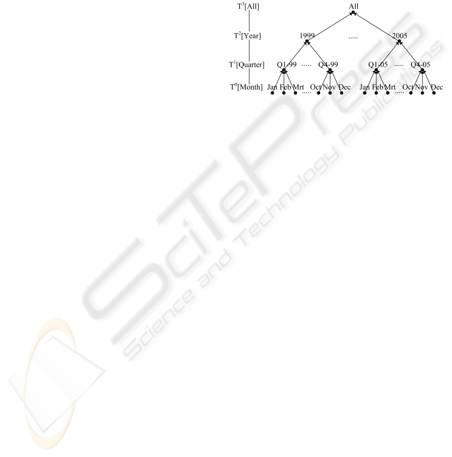
the Time dimension is depicted in Figure 1.
Figure 1: The left-side represents the hierarchy schema
of the Time dimension; the right-hand side represents the
rooted tree of its dimension hierarchy instances.
With each dimension hierarchy in domain D
k
a
rooted tree T (D
k
) = (V, E) is associated, called the
dimension hierarchy tree of D
k
, depicted in Figure 1
right.
The instance element d
i
k
+1
k
∈ D
i
k
+1
k
is called a par-
ent and d
i
k
k
∈ D
i
k
k
is called its child. In the tree the year
1999 is the parent of the children {1999.Q1, 1999.Q2,
1999.Q3, 1999.Q4}, for example. To determine the
parent of some child element in the hierarchy of a
single domain D
i
k
k
, we define a 1-dimensional roll-up
operator as:
r
+1
(d
i
k
k
) = d
i
k
+1
k
, (2)
and reversely, to determine the children of some par-
ent element in the hierarchy, a 1-dimensional drill-
down operator is defined as:
r
−1
(d
i
k
k
) = d
i
k
−1
k
. (3)
These operators r
+1
and r
−1
can also be applied on
any subset X
i
k
k
of D
i
k
k
, and the operators can be ap-
plied both on the schema as on the instance level.
For example, on the schema level as r
−1
(T
2
[Year]) =
T
1
[Quarter], or on the instance level as r
−1
(1999), to
determine the children of some specific year.
2.2 Cubes and Cells
The key structure in the multi-dimensional database
is the data cube. A cube or a sub cube C is defined as
the Cartesian product over the levels of the available
domains:
X
i
1
1
× X
i
2
2
× . . . × X
i
n
n
, where X
i
k
k
⊆ D
ik
k
. (4)
WHAT-IF ANALYSIS IN OLAP - With a Case Study in Supermarket Sales Data
209

For example, Time
1
× Store Region
1
× Product
3
,
T
1
× S
1
× P
3
, and so on, are cubes in the case study.
Note that according to this definition also a single di-
mension hierarchy is composed out of cubes, e.g. the
left hand side of Figure 1 shows the cubes that make
up the Time dimension. An alternative representa-
tion of a full cube is given by (D
i
1
1
, D
i
2
2
, . . . , D
i
n
n
), or
as [i
1
, i
2
, . . . , i
n
] in shorthand notation.
A cell is defined as an instance element of a cube
X
i
1
1
× X
i
2
2
× . . . × X
i
n
n
:
(d
1
, d
2
, . . . , d
n
), (5)
where d
1
∈ X
i
1
1
, d
2
∈ X
i
2
2
, . . ., d
n
∈ X
i
n
n
. Accordingly,
a cell contains a single instance value for each of its
domains. For example, (2000.Q1, Vancouver, Food)
is a cell in the example cube Time
1
×Store Region
1
×
Product
3
.
In addition, the instances at the lowest dimension
levels of each of its domains [0, 0, . . . , 0] are cells of
the base cube D
0
1
× D
0
2
× . . . × D
0
n
, labelled as C
B
. For
example, in the financial database the base cube is
represented by Time
0
× Store Region
0
× Product
0
.
The base cube can be aggregated to a higher hierar-
chical level in the domain by applying roll-up oper-
ators (see Section 2.3). When all dimension hierar-
chies are aggregated at the highest level, we derive the
0-dimensional top cube D
i
max
1
1
× D
i
max
2
2
× . . . × D
i
max
n
n
,
labelled as C
T
. The top cube consists of only one cell
(All, All, . . . , All).
2.3 Navigational Operators
A number of navigational operations are available to
the business analyst to manual explore OLAP cubes,
allowing interactive querying and analysis of the data.
In this paper, we redefine these navigational opera-
tions on cubes, i.e. on multiple dimensions, in our
notation. The operations are defined on the domains
of the cube C as in equation (4). Thus, these oper-
ations also hold for full cubes where X
i
q
q
= D
i
q
q
and
cells where X
i
q
q
= d
i
q
q
, since these are simply special
cases of the sub cube. The most important naviga-
tional operations or queries for cubes are:
Drill-down, which de-aggregates a cube to a lower
dimension level, is defined as:
R
−1
q
(X
i
1
1
× . . . × X
i
q
q
× . . . × X
i
n
n
) =
X
i
1
1
× . . . × r
−1
(X
i
q
q
) × . . . × X
i
n
n
.
(6)
For example, a drill-down operation on the Time hi-
erarchy from the level Year to the level Quarter, in
the example full cube R
−1
Time
(Time
2
× Store Region
3
× Product
2
) results in the full cube Time
1
× Store
Region
3
× Product
2
.
Roll-up, the reverse of drill-down, which aggre-
gates a cube along one or more dimension hierarchies
to a higher dimension level, is defined as:
R
+1
q
(X
i
1
1
× . . . × X
i
q
q
× . . . × X
i
n
n
) =
X
i
1
1
× . . . × r
+1
(X
i
q
q
) × . . . × X
i
n
n
.
(7)
Obviously, drill-down and roll-up (6) and (7)
are the inverse of each other: R
+1
q
(R
−1
q
(C)) =
R
−1
q
(R
+1
q
(C)) = C.
We refer to (Han and Kamber, 2005) for an elabo-
rate overview on navigational operators.
2.4 Aggregation Lattice
By rolling-up the full base cube D
0
1
×D
0
2
×. . . ×D
0
n
, or
one of its sub cubes X
0
1
× X
0
2
× . . . × X
0
n
, over several
associated dimensions and dimension hierarchies, in
any order, a lattice of cubes L is formed. This lattice
L has at the bottom the base cube [0, 0, . . . , 0] and at
the top the cube [i
1
, i
2
, . . . , i
n
], and is defined by the
following sequence of operations, applied to the base
cube:
R
+i
1
1
◦ R
+i
2
2
◦ . . . ◦ R
+i
n
n
(D
0
1
× D
0
2
× . . . × D
0
n
) =
D
i
1
1
× D
i
2
2
× . . . × D
i
n
n
,
(8)
where R
+n
q
= R
+1
q
◦. . . ◦R
+1
q
. The complete lattice has
[i
max
1
, i
max
2
, . . . , i
max
n
] at the top. Note that by com-
mutativity of the roll-up operators the different orders
of application yield the same result. Moreover, as a
result of its definition, the lattice structure holds for
full cubes, sub cubes, and cells, that might be derived
from the multi-dimensional database.
With the concept of the aggregation lattice, we
define the parents and children of a cube C. A
parent cube C
0
in L is defined as the result of the
roll-up operation R
+1
q
(C) = C
0
. Obviously, a par-
ent cube might have multiple child cubes, for exam-
ple, the parent cube [i
1
, i
2
, . . . , i
n
] has [i
1
−1, i
2
, . . . , i
n
],
[i
1
, i
2
− 1, . . . , i
n
], . . ., [i
1
, i
2
, . . . , i
n
− 1] as its child
cubes. Reversely, to determine all the child cubes
of cube C in the lattice, we have to apply a drill-
down operation on all its associated domains. Ob-
viously, due to the lattice structure, a child cube usu-
ally has multiple parents, for example, the child cube
[i
1
, i
2
, . . . , i
n
], has [i
1
+ 1, i
2
, . . . , i
n
], [i
1
, i
2
+ 1, . . . , i
n
],
. . . , [i
1
, i
2
, . . . , i
n
+ 1] as is parent cubes, correspond-
ing to the different roll-ups. In addition, in the lattice
the partial ordering within the dimension hierarchies
is preserved.
We define, the upset of a cube C = [i
1
, i
2
, . . . , i
n
] is
the lattice of all ancestors of the cube C. The upset of
a cube C is a sub lattice of the complete lattice, with
the base cube C and top [i
max
1
, i
max
2
, . . . , i
max
n
]. It is
ICEIS 2010 - 12th International Conference on Enterprise Information Systems
210

obtained by applying roll-up operations on the cube
C repeatedly, in any order. The downset of a cube
C = [i
1
, i
2
, . . . , i
n
] is the lattice of all descendants of
the cube C. The downset of a cube C = [i
1
, i
2
, . . . , i
n
]
is the sub lattice of the complete lattice with base cube
[0, 0, . . . , 0] and top C. It is obtained by applying drill-
down operations on the the cube C repeatedly, in any
order. The upset and downset of a single cell are de-
fined similarly.
An analysis path P is defined as a sequence of p
drill-down (roll-up) operators, as defined in equation
(7), executed over the cubes of the lattice. The length
of a path from the cube [i
1
, i
2
, . . . , i
n
] somewhere in the
lattice to the base cube [0, 0, . . . , 0] is i
1
+ i
2
+ . . . + i
n
.
Obviously, the sum of the indices of a cube corre-
sponds with the number of aggregations carried out,
i.e. the level of L under consideration.
2.5 Measures
Measures are derived from the column names of the
fact table, and its measure values. The instances of
the measures, are entries of the fact table. A measure
y is defined as a function on a cube C:
y
i
1
i
2
...i
n
: D
i
1
1
× D
i
2
2
× . . . × D
i
n
n
→ X. (9)
where measure values are, for example, X = N, Z, or
R. We also use the word variable instead of measure.
Data are the values of a measure y in a partic-
ular cell like, for example, sales
232
(2000, Canada,
Food)= 70, 028. The combination of a cell and a mea-
sure is called a data point. The measure’s upper index
indicates the level of the cell on the associated dimen-
sion hierarchies. Furthermore, if a measure is not de-
fined for a particular cell, we call the cell an empty
cell.
If a measure is related to the base cube [0, 0, . . . , 0],
then the dimension hierarchies of the domains
can be used to aggregate the measure values of
y
00...0
(d
1
, d
2
, . . . , d
n
) by typical aggregation functions
like SUM(), COUNT(), MAX(), MIN(), or AVG().
3 ADDITIVE MEASURES
The measure y
i
1
...i
q
...i
n
is defined as a additive mea-
sure, in the terminology of (Lenz and Shoshani,
1997), if for each cube C in the lattice L(y), except
the base cube, the following holds:
y
i
1
...i
q
...i
n
(C) =
∑
q
y
i
1
...(i
q
−1)...i
n
(R
−1
q
(C)). (10)
Equation (10) also holds for all individual cells in the
cube.
From our case study database, we could inspect
the measure sales as a function on the sub cube C,
given by 2000 × Store Country × Product Family.
This cube is part of the lattice L(sales), formed by
rolling-up with the SUM() aggregation function. By
applying equation (10) two times we get:
sales
242
(C) =
∑
k
sales
142
(R
−1
Year
(C)) =
∑
l
∑
k
sales
132
(R
−1
Store Region
(R
−1
Year
(C))).
For the cell (2000, All-Regions, Food) in C, an instan-
tiated equation corresponding to the above drill-down
operations reads:
sales
242
(2000, All-Regions, Food) =
4
∑
j=1
3
∑
k=1
sales
132
(2000.Quarter
j
, Store Country
k
, Food),
where S
j
(2000.Quarter) = 2000.Quarter
j
. Further-
more, the additive COUNT() function is defined simi-
larly, and treated as a special case of the SUM() func-
tion, only this operator summarizes dimension hierar-
chy instances instead of measure instances.
4 WHAT-IF ANALYSIS
Now we want to investigate the influence of a
change in a measure value of a cell, in any cube
on a higher level value of the same measure. Or
in formal notation, what would be the change
in y
j
1
j
2
... j
n
(d
j
1
1
, d
j
2
2
, . . . , d
j
n
n
) if the measure value
y
i
1
i
2
...i
n
(d
i
1
1
, d
i
2
2
, . . . , d
i
n
n
) in a cube at a lower level is
changed by the amount δ, keeping all other measure
values in the cube [i
1
, i
2
, . . . , i
n
] unchanged. To solve
this we consider the lattice L of cubes with base cube
[i
1
, i
2
, . . . , i
n
] and top cube [ j
1
, j
2
, . . . , j
n
]. The values
of the measure y in the cube [i
1
, i
2
, . . . , i
n
] are denoted
by x(d
1
, d
2
, . . . , d
n
) and y(d
1
, d
2
, . . . , d
n
) in the higher
level cubes of [ j
1
, j
2
, . . . , j
n
]. We distinguish between
the original values of a measure without change x
r
and
y
r
, and the values of the changed measure: x
a
and y
a
,
where x
a
= x
r
except for one cell c
0
in the base cube,
and δ = x
a
− x
r
.
Theorem 1. There is a unique additive measure y
a
defined on all cubes in the lattice L such that:
y
a
(c) = y
r
(c) + β(c) · (x
a
− x
r
), (11)
where:
β(c) = 1 if c
0
is a descendant of c, and
β(c) = 0 if c
0
is not a descendant of c.
WHAT-IF ANALYSIS IN OLAP - With a Case Study in Supermarket Sales Data
211

Proof. To show that y
a
is additive it is sufficient to
show that β(c)· (x
a
− x
r
) is additive, because the sum
of additive measures is also additive and y
r
is additive.
Thus, we must show that:
β(c) =
∑
q
β(R
−1
q
(c)), (12)
where R
−1
q
is a drill-down operator defined on a cube
or cell in the lattice L. Now there are two cases:
case 1) c
0
is a descendant of c. In that case c
0
is
also a descendant of R
−1
q
(c), which are the children of
c in direction q. This property does not depend on q.
So both sides of equation (12) are equal to 1.
case 2) c
0
is not a descent of c. But in that case,
it also not a descendant of the children of c. Hence,
both sides of equation (12) are zero.
It is important to note that, for any cell c
0
in the
base cube of a lattice, that if cell c
0
is a descendant of
R
−1
q
1
(c) then it is also a descendent of R
−1
q
2
(c).
Note that the measure y
a
is unique. This follows
from the general proposition that every additive mea-
sure with given values on the base cube is unique.
To show this, now suppose that we have a (sub) lat-
tice L with top cube C = [ j
1
, j
2
, . . . , j
n
] and base cube
C
0
= [i
1
, i
2
, . . . , i
n
]. In the lattice the drill-down opera-
tors are commutative, different orders of application,
over all analysis paths from top to base, give the same
cube. Or stated formally:
R
− j
1
1
◦ R
− j
2
2
◦ . . . ◦ R
− j
n
n
(C) =
R
− j
n
n
◦ . . . ◦ R
− j
2
2
◦ R
− j
1
1
(C) = C
0
.
(13)
This property together with equation (10) ensures that
the system of additive equations, represented in L has
a unique solution if the measure is defined on the base
cube.
Now the what-if analysis can be carried out as fol-
lows. If a base cell x
a
(d
1
, d
2
, . . . , d
n
) is changed with
some δ, all elements in its upset are changed with that
δ. This follows immediately from Theorem 1.
5 SOFTWARE
IMPLEMENTATION
Our prototype software is implemented in MS Ex-
cel/Access in combination with Visual Basic, see
(Caron and Daniels, 2009) for a detailed overview of
the core functionality. For the implementation of the
ideas in this paper we build on this functionality. The
software connects with an OLAP database in MS Ac-
cess. In MS Excel a cube can be constructed from
this database and inspected via a pivot table. In such
a pivot table, the analyst can do what-if analysis on
a specific cell, by selecting the cell and pushing the
analysis button. Now the analyst can decide to change
the cell with some percentage or absolute value, see
Figure 2. The result will be that the original cell value
and its upset are changed with that value. In the soft-
ware all changed cells are indicated with a color, see
Figure 3. Next the analyst might decide to do a new
analysis and build on the previous one, or he might
undo his action to return to the original pivot table.
After some actions the analyst can always return to
the original situation because all operations are exe-
cuted on a (virtual) copy of the OLAP database. Obvi-
ously, in the software only the modified cell, in some
cube in the lattice, and its changed upset need to be
stored for a single analysis.
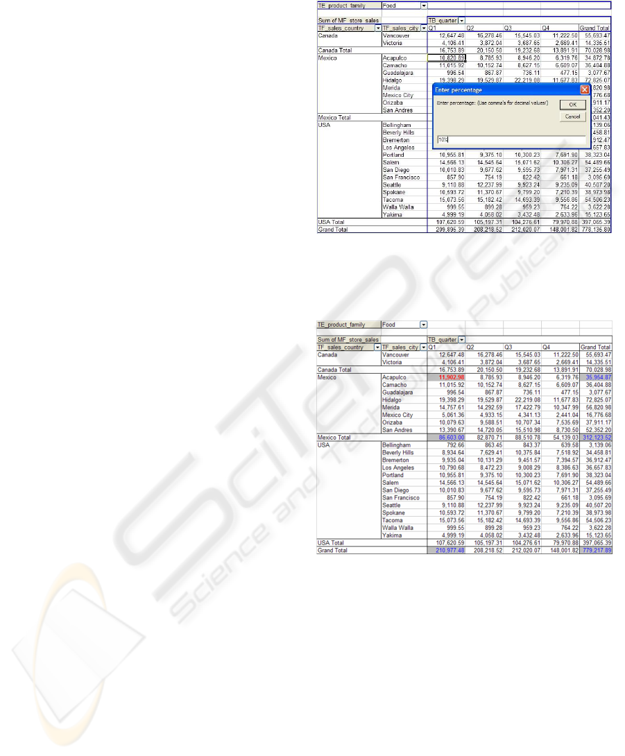
6 CASE STUDY: SUPERMARKET
SALES DATA
In this section we apply our prototype analysis soft-
ware on an artificial but realistic supermarket sales
data set, modelled as a star scheme. The data set has
164, 558 records in the sales fact table for the year
2000 for supermarkets in North America, with mea-
sures as sales, costs, revenues, and so on. Typical di-
mensions with hierarchies in the data set are: Time
(see Section 2.1 for the hierarchy), Store Region (with
hierarchy: Store Name ≺ Store City ≺ Store Region
≺ Store Country), Product (with hierarchy: Product
Name ≺ Product Sub-Category ≺ Product Category
≺ Product Family), etc.
In the data set we have the lattice with base cube
Month × Store Name × Product Name or [0, 0, 0]
and with top cube All-Times × All-Stores × All-
Products or [3, 4, 4]. Now suppose we are inspect-
ing the cube Year.Quarter × Country.City × Prod-
uct Family or [1,1,3], with slices on Year = 2000 and
Product Family = ‘Food’ with the additive measure
store sales. In the cube we want analyse the impact of
a 10% increase in the cell store sales(2000.Q1, Mex-
ico.Acapulco, Food)= 10, 820.89 on its upset cells in
[2,1,3], [1,2,3], [2,2,3], and [2,4,3], see Figure 2 in the
Appendix, where a number screenshots are depicted
from our software.
The result of this analysis is depicted in Fig-
ure 3, where the colored cells (with grey) indicate
the changed cells in its upset, that is partly visu-
alized, with δ = 1082.09. For example, the value
of the top cube changes to store sales
a
(2000, All-
Countries, Food)= 779, 217.89 from its original value
778, 135.80. Obviously, the part of the upset that is
not visualized in the figures is also updated. If, for ex-
ample, the cube (2000.Quarter, Country.Region.City,
Food), also noted as [2,3,3], one would observe the
ICEIS 2010 - 12th International Conference on Enterprise Information Systems
212
impact of the induced change. This clearly shows,
that the what-if analysis takes place in a full OLAP
environment, with full support of OLAP’s naviga-
tional operators, and not in a static reporting environ-
ment. This clearly is of benefit to the OLAP analyst.
REFERENCES
Cariou, V., Cubill
´
e, J., Derquenne, C., Goutier, S., Guisnel,
F., and Klajnmic, H. (2008). Built-in indicators to dis-
cover interesting drill paths in a cube. In DaWaK ’08:
Proceedings of the 10th international conference on
Data Warehousing and Knowledge Discovery, pages
33–44, Berlin, Heidelberg. Springer-Verlag.
Caron, E. and Daniels, H. (2008). Extensions to the
olap framework for business analysis. In ICSOFT
(ISDM/ABF), pages 240–247.
Caron, E. and Daniels, H. (2009). Business analysis in the
olap context. In ICEIS (2), pages 325–330.
Caron, E. A. M. and Daniels, H. A. M. (2007). Explana-
tion of exceptional values in multi-dimensional busi-
ness databases. European Journal of Operational Re-
search, 188:884–897.
Daniels, H. A. M. and Caron, E. A. M. (2009). Automated
explanation of financial data. Intelligent Systems in
Accounting, Finance & Management, 16(1-2):5–19.
Han, J. and Kamber, M. (2005). Data Mining: Concepts
and Techniques. Morgan Kaufmann Publishers Inc.,
San Francisco, CA, USA.
Lenz, H. J. and Shoshani, A. (1997). Summarizability in
OLAP and statistical data bases. In Statistical and
Scientific Database Management, pages 132–143.
Sarawagi, S., Agrawal, R., and Megiddo, N. (1998).
Discovery-driven exploration of olap data cubes. In
Conf. Proc. EDBT ’98, pages 168–182, London, UK.
Springer-Verlag.
APPENDIX
Figure 2: Here we anticipate on a 10% increase in the cell
store sales(2000.Q1, Mexico.Acapulco, Food)= 10, 820.89
in the cube (2000.Quarter, Country.City, Food). This
change is automatically propagated to its upset cells.
Figure 3: Result of the what-if analysis in the cube
(2000.Quarter, Country.City, Food). Colors indicate the
changed cells in the upset.
WHAT-IF ANALYSIS IN OLAP - With a Case Study in Supermarket Sales Data
213
