
AN EXTENSIBLE ENSEMBLE ENVIRONMENT FOR TIME
SERIES FORECASTING
Claudio Ribeiro, Ronaldo Goldschmidt and Ricardo Choren
Department of Computer Engineering, Military Institute of Engineering, Rio de Janeiro, RJ, Brazil
Keywords: Time Series Forecasting, Ensembles, Software Tool, Data Mining.
Abstract: There have been diverse works demonstrating that ensembles can improve the performance over any
individual solution for time series forecasting. This work presents an extensible environment that can be
used to create, experiment and analyse ensembles for time series forecasting. Usually, the analyst develops
the individual solution and the ensemble algorithms for each experiment. The proposed environment intends
to provide a flexible tool for the analyst to include, configure and experiment with individual solutions and
to build and execute ensembles. In this paper, we describe the environment, its features and we present a
simple experiment on its usage.
1 INTRODUCTION
A time series is a time-ordered sequence of
observation values of a variable made at equally
spaced time intervals Dt, represented as a set of
discrete items x
1
, x
2
, ..., etc (Palit and Popovic,
2005). Time series prediction idea is to forecast
(with the best accuracy possible) future unknown
data values based on historical patterns in the
existing data. There are several approaches to time
series forecasting, such as moving average,
exponential smoothing, ARIMA (Box and Jenkins,
1970), and fuzzy logic (Wang and Mendel, 1992).
It is generally accepted that individual models
for time series forecasting are usually unable to
produce satisfactory results (Wang et al., 2005).
Thus it is natural to consider combining multiple
models to generate better data forecasting. Such a
combined system is commonly referred as an
ensemble (Bouchachia and Bouchachia, 2008).
There are several ways to combine base models
predictions in an ensemble. However, the majority
of ensemble applications use several variations
(configurations) of only one base model method.
The ensemble combination method is used to bring
about diversity in the base models’ predictions.
There has been little work (e.g., (Merz, 1999)) on
creating ensembles that use many different types of
base models. This paper presents an environment for
ensemble configuration and execution. It allows the
analyst to use several base model methods to make a
forecast.
The rest of this paper is organized as follows.
Sections 2 and 3 respectively present de DMEE and
its prototype. Section 4 shows an usage example and
section 5 concludes this paper.
2 THE DMEE
This section describes a flexible environment for the
configuration and execution of ensembles, called
Data Mining Ensemble Environment (DMEE). The
DMEE is designed as a framework to allow
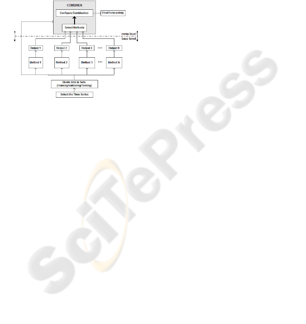
extensibility. Figure 1 shows the DMEE general
architecture. It allows the selection of time series;
the configuration (inclusion/exclusion and selection)
of base model methods; the execution of configured
base model methods; the configuration of
combination model methods, and; the selection of
metrics to evaluate the performance of the devised
ensemble. The following subsections describe the
general process underlying the DMEE.
2.1 Time Series Selection
The analyst should begin by selecting the time
series. Thus the analyst indicates the database with
the time series and she selects the attributes (one to
be predicted and another to indicate the time
ordering). Then, the available data are divided into
404
Ribeiro C., Goldschmidt R. and Choren R. (2010).
AN EXTENSIBLE ENSEMBLE ENVIRONMENT FOR TIME SERIES FORECASTING.
In Proceedings of the 12th International Conference on Enterprise Information Systems - Artificial Intelligence and Decision Support Systems, pages
404-407
Copyright
c
SciTePress
three possible set: training set, validating set and
testing set. This feature allows the analyst to define
the sets that will be used by the ensemble (meta)
method. The base model methods will use the same
sets which were defined for the ensemble. The
DMEE does that to avoid biasing for either a base
model method or for the ensemble method.
Figure 1: The DMEE general architecture.
2.2 Base Model Method Execution
and Selection
After selecting the time series and the dividing its
data into the appropriate sets for the ensemble, the
analyst should configure and execute the base model
methods chosen from the repository to be used in the
ensemble. The DMEE core functionality executes
each base model method each one at a time and it
stores the prediction results in a database. These
results will be used as input for the ensemble
combination method.
It is interesting to mention that, since the DMEE
stores a base model method result, this result can be
used anytime later. The execution of a method is
very time consuming and, in the current version of
the DMEE, there is no concurrency. The idea behind
this feature is to save time by trying to reuse the
results of a particular method execution (i.e. a
specific base model method configuration).
After executing the base model methods, the
analyst can verify their performance (based in
whichever criteria the analyst desires). To improve
the ensemble results, she can select which base
model methods will build the ensemble. The DMEE
provides five approaches for base model methods
selection: (i) all methods: the results from all the
base model methods executed will be used in the
ensemble combination method; (ii) individual
selection: the analyst can choose which base model
method results will be used in the ensemble
combination method; (iii) selection by maximum
index: the analyst indicates a maximum error value
for the base model method results. The DMEE will
select those base model methods that present a
prediction error smaller than the value provided by
the analyst; (iv) selection by percentage index: this
approach is similar to the above. The difference is
that the metric used to analyze the base model
method performance does not indicate an absolute
error, but rather a percentage error; (v) automatic
selection (based on simple averaging combination):
this approach allows the DMEE to automatically
select the set of base model method results to be
used in the ensemble by executing a series of
simulations to evaluate the combination of the
obtained results.
2.3 Combination Method Selection
and Execution
After selecting which base model methods will be
used in the ensemble, the analyst should select the
combination method. The DMEE provides two types
of combination methods: linear and non-linear. The
available linear combination methods are simple
averaging and weighted averaging. If the analyst
chooses to use non-linear combination, she can use
any method (from the DMEE repository) to combine
the base model method results. In the DMEE, the
analyst can configure two strategies for the
combination method: combination and training. The
idea is to let the analyst execute several possibilities
for the same ensemble method.
The combination strategies are: (i) simple
combination: only the results of the base model
methods are used as input for the combination
method; (ii) compound combination: besides the
results of the base model methods, the original time
series is used as input for the combination method.
The training strategies are: (i) single phase training:
the composition method uses only the training set;
(ii) two phase training: the composition method uses
both the training and the validation sets.
The DMEE executes the combination method
and stores its results for analysis purposes. The
execution of the combination method has a
particular issue when the base model methods use
the prediction window concept (e.g. regression
methods). The prediction windows of the base
model methods should be aligned to indicate the
initial time index to be used in the training phase of
the combination method. If the combination method
AN EXTENSIBLE ENSEMBLE ENVIRONMENT FOR TIME SERIES FORECASTING
405

itself uses a prediction window, this window should
be considered in the alignment.
2.4 Result Analysis
The analyst can make a result analysis. The analyst
selects metrics to view the performance of the base
model methods and of the composition method. The
results are shown graphically to the analyst.
3 THE DMEE PROTOTYPE
The current version of the DMEE prototype was
developed using Java. To start using the DMEE tool
(including the base model methods already
imported) for forecasting, the analyst must select a
time series. The original data of the time series must
be stored in a database.
After selecting the time series to forecast, the
analyst should configure the training, validation and
testing subsets (figure 2). This configuration will be
used by the DMEE to execute the code for each
selected base model method. As mentioned, the
methods are executed one at a time and their results
are stored for future reuse.
Figure 2: Subset configuration.
Then, the analyst can select the base model
methods results that will be used as input for the
ensemble method. This selection can be done using
one of the five approaches listed in section 2.2.
Currently, the metrics that can be used in the
selection by maximum index and selection by
percentage index are: U-Theil, mean square error,
root mean square error, sum of squares error, mean
absolute error and mean absolute percentage error.
The analyst must configure the ensemble method
(figure 3). The DMEE prototype executes the
ensemble method and stores its results in a database.
These results can be analyzed to compare the
performances of the individual base model methods
with the ensemble method.
Figure 3: Ensemble configuration (linear and non-linear).
4 A SAMPLE STUDY
This section presents an experiment on using the
DMEE environment for the prediction of the
Mackey-Glass (Wan, 2009) time series. The data
used encompassed 1500 records, the lowest series
value was 0.212559300 and the highest series value
was 1.378507200.
In this study, all available base model methods
were used. The configurations were:
i. Naive Forecasting: no configuration needed
ii. Exponential Smoothing: smoothing factor = 0.9
iii. Moving Average: prediction window = 3
iv. Wang-Mendel: prediction window = 7; number
of fuzzy sets = 7
v. Backpropagation: learning rate = 0.6;
momentum factor = 0.3; number of epochs =
5.000
a. Input layer: # of neurons = 9; activation
function = linear
b. Hidden layer: # neurons = 9; activation
function = sigmoid
c. Output layer: # neurons = 1; activation
function = linear
Table 1 shows the results for the base model
methods executions, using the configurations
depicted above. The backpropagation method gave
the best results while the Moving Average presented
the worst results. Figure 4 shows the results for an
ensemble using a non-linear combination configured
with a backpropagation method. The ensemble used
all base model method results. In this scenario (all
ICEIS 2010 - 12th International Conference on Enterprise Information Systems
406

Table 1: Base model methods results.
Figure 4: Ensemble results.
base model methods and backpropagation) the
ensemble results were only slightly better than the
results achieved by the base model methods.
5 CONCLUSIONS
This paper has presented an extensible environment
for experimentation in time series forecasting using
ensemble approaches in conjunction with popular
forecasting methods. The idea is to provide a tool to
configure and test several ensemble options. The
DMEE allows for base model methods extension,
ensemble configuration and base model method
results persistence. The diversity of information
required to configure base methods and ensembles
were summarized for simplicity.
It was not our intention in this work to run
experiments to compare single base model method
results with ensemble results. The main purpose of
this work is to show an environment to help analysts
try ensemble approaches for time series forecasting.
REFERENCES
Bouchachia, A. and Bouchachia, S., 2008. Ensemble
learning for time series prediction. In Proceedings of
the International Workshop on Nonlinear Dynamic
Systems and Synchronization.
Box, G. E. P. and Jenkins, G. M., 1970. Time series
analysis: forecasting and control. Holden-Day.
Merz, C. J., 1999. A principal component approach to
combining regression estimates. Machine Learning,
36:9–32.
Palit, A. K. and Popovic, D., 2005. Computational
intelligence in time series forecasting: theory and
engineering applications. Springer-Verlag.
Wan, E. A., 2010. Time series data. Department of
Computer Science and Electrical Engineering. Oregon
Health & Science University (OHSU), available at
http://www.cse.ogi.edu/~ericwan/data.html
Wang, L. X. and Mendel, J. M., 1992. Generating fuzzy
rules by learning from examples. IEEE Transactions
on Systems, Man and Cybernetics, 22(6):1414–1427.
Wang, W., Richards, G., and Rea, S., 2005. Hybrid data
mining ensemble for predicting osteoporosis risk. In
Proceedings of the 27th IEEE Engineering in
Medicine and Biology Conference, pages 886–889.
AN EXTENSIBLE ENSEMBLE ENVIRONMENT FOR TIME SERIES FORECASTING
407
