OFFROAD NAVIGATION USING ADAPTABLE MOTION PATTERNS

Frank Hoeller, Timo R

ohling and Dirk Schulz

Fraunhofer Institute for Communication, Information Processing and Ergonomics FKIE, Germany

Keywords:

Outdoor robotics, Local navigation, Motion patterns, Motion templates, Motion learning.

Abstract:

This paper presents a navigation system which is able to steer an electronically controlled ground vehicle to

given destinations considering all obstacles in its vicinity. The approach is designed for vehicles without a

velocity controlled drivetrain and without an odometry system, making it especially useful for typical remote-

controlled vehicles without upgrading the motor controllers. The vehicle is controlled by sets of commands,

each set representing a speciﬁc maneuver. These sets are then combined in a tree-building procedure to form

trajectories towards the given destination. While the sets of commands are executed the vehicle’s movement

is measured to reﬁne the prediction used for path generation. This enables the approach to adapt to surface

alterations. The technique requires a precise position estimation, which is provided in our implementation by

a 3D laser mapping based relative localization system. We tested our approach using a 400kg EOD robot in

an outdoor environment. The experiments conﬁrmed that our navigation system is able to control the robot to

its destination while avoiding obstacles and adapting to different ground surfaces.

1 INTRODUCTION

In the design of robot systems operating in unstruc-

tured outdoor environments, special care has to be

taken that the robots do not accidentally collide with

obstacles in their vicinity. Compared to indoor situ-

ations the robot can suffer drastically more damage

by the more hazardous surrounding. Safe operation

is commonly achieved by means of collision avoid-

ance mechanisms which ensure a minimal distance

to obstacles. This task is exacerbated by different

ground surfaces which have a distinct effect on the

wheel grip. This deviation has to be anticipated to en-

sure the reproducibility of planned motions and thus

making collision avoidance possible.

Additional complications arise for robots which

were designed for remote-control. Such robots are

normally only equipped with relatively simple mo-

tor controllers. This has a signiﬁcant impact on the

techniques available for the collision avoidance be-

cause most classic navigation algorithms only gener-

ate velocity commands. To interpret such commands

the controllers need to have an appropriate servo loop,

which is not the case for such robots.

In this article we present an approach which al-

lows a mobile robot with any kind of electronic mo-

tor controller to operate in cluttered outdoor environ-

ments. To be able to improve the navigation behavior

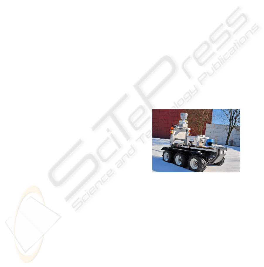
Figure 1: The Quinetiq Longcross robot Suworow equipped

with a Velodyne 3D and an additional (unused) 2D laser

range ﬁnder.

of the robot in unknown locations, our approach fol-

lows a local navigation paradigm and does not need a

map of the environment. Instead, the robot’s motion

control decides solely based on the robot’s sensory in-

put; in our current implementation this is a Velodyne

3D laser range scanner with 360 degree ﬁeld of view

which is used to compute a local 2.5D map. In ad-

dition, the laser scanner is used to exactly determine

the robot position in a local frame of reference using

a local mapping technique. This procedure also com-

pensates the missing robot odometry.

The motion planning for the robot is based on a

tree-search technique which we developed to suit the

special requirements of the robot’s motor controllers.

Our planning algorithm composes paths by combin-

186

Hoeller F., Röhling T. and Schulz D. (2010).

OFFROAD NAVIGATION USING ADAPTABLE MOTION PATTERNS.

In Proceedings of the 7th International Conference on Informatics in Control, Automation and Robotics, pages 186-191

DOI: 10.5220/0002916301860191

 SciTePress

ing predeﬁned Motion Patterns. Each Motion Pat-

tern consists of a set of robot commands and a se-

ries of poses which represent the robot’s movement

when the command set is executed by the controllers.

With these Motion Patterns, the local navigation mod-

ule repeatedly computes trees of collision-free com-

mand sequences. From each tree a path is extracted

which brings the robot close to the destination coordi-

nate as fast as possible. To tackle the surface traction

problem, the robot’s movements are measured on the

ﬂy. The collected data is used to update the measured

movement part of the Motion Patterns. The upgraded

Motion Patterns are handed over to the planning pro-

cess and used for the tree generation.

The remainder of this article is organized as fol-

lows: After discussing related work in section 2, we

introduce our Velocity Grid environment representa-

tion in section 3 followed by a description how they

are utilized by our Motion Pattern based local navi-

gation approach in Section 4. Section 5 then explains

the movement measuring and Motion Pattern learning

procedures. Before we conclude, we describe some

experiments carried out with our robot to illustrate the

capabilities and the robustness of our approach. We

implemented our approach on a Quinetiq Longcross

EOD robot (see Figure 1) and veriﬁed its feasibility

in outdoor settings.

2 RELATED WORK

Waypoint navigation is one of the fundamental tasks

for autonomous mobile robots. Many popular sys-

tems utilize the beneﬁts of cars with ackermann steer-

ings by ﬁrst generating a feasable path and then try to

follow this path as fast as possible. This can be done

because, apart from physical limitations of the vehi-

cle, the velocity does not affect the trajectory. For ex-

ample, the DARPA Grand Challenge winning robot

Stanley (Thrun et al., 2006) beneﬁts from this prin-

ciple. But because our robot does not have a veloc-

ity controlled drivetrain, the velocity cannot be con-

trolled without affecting the trajectories.

Another approach (V. Hundelshausen et al., 2008)

uses a different navigation technique by deﬁning

a limited set of commands or command-sequences

and greedily decides in every computing interval

which entity should be applied. Their path genera-

tor uses combinations of speeds and steering angles

to generate trajectories which are then further eval-

uated. Therefor, an occupancy grid generated by a

3D-laser and different weighting functions are used.

This is similar to the Dynamic Window Approach

(DWA) (Fox et al., 1997; Brock and Khatib., 1999)

because both methods restrict the search to a single

time step, i.e. they select the next best controls based

on the current sensor input and a model of the robot’s

dynamics.

In addition to these pure navigation algorithms,

learning methods for robot motion have also been pro-

posed in the past. Future robot positions can be es-

timated by regarding the current terrain type (Brun-

ner et al., 2010). Therefor, intertial sensor data is

processed with Gaussian process models to infer the

movement velocities for position estimation and to

deduce the terrain type from vibrations. Unfortu-

nately, this method can only distinguish known sur-

faces and the used models require large amounts of

computational power. Gaussian Processes in com-

bination with reinforcement learning have been used

to predict the movement of autonomous blimps (Ko

et al., 2002), but just as the approach above it requires

an extensive preparation phase. Seyr et al. use arti-

ﬁcical neural networks to predict the trajectories of a

two-wheeled robot (Seyr et al., 2005). It was shown

that every trained situation can be recognized by their

predictor. The used robot model is heavily bound to

velocity parameters and thus again requires a suitable

drivetrain.

The concept of motion template based learning

has been previously employed to simplify the learn-

ing of complex motions (Neumann et al., 2009). In

contrast to our approach the templates have param-

eters which are adjusted to ﬁt the desired trajectory.

This implies a feasible correlation between parameter

input and drivetrain behavior.

3 VELOCITY GRIDS

In outdoor environments, a 3D-sensor (see Figure 1)

is indispensable for an effective collision avoidance.

Commonly used two-dimensional indoor variants are

almost useless because of their insufﬁcient envi-

ronment coverage. However, the gain in coverage

comes with the disadvantage of a drastically increased

amount of data. Processing all this information while

planning motions requires an unreasonable amount of

computing power. Thus we simplify the 3D-sensor’s

data to a two-dimensional grid. In every grid cell the

maximum admissible velocity of the corresponding

area is stored. This type of map is referred to as Ve-

locity Grid and it can be used for collision tests with

less operating expense. This allows us to use modi-

ﬁed two-dimensional planning algorithms. Although

Velocity Grids seem to be similar to costmaps, they

are utilized by our local navigation algorithm in a dif-

ferent way (see section 4).

OFFROAD NAVIGATION USING ADAPTABLE MOTION PATTERNS

187

Figure 2: Left: A 2.5D height map acquired using a Velo-

dyne. Right: The corresponding Velocity Grid. A car and

the following person are marked as impassable (red), the

sidewalk’s curb is identiﬁed as slowly traversable (yellow).

To generate a Velocity Grid, the ﬁrst step is to cal-

culate a 2.5D map or height grid. A simple method

to do this is to use a maximum-function on all mea-

surements corresponding to one cell. Of course more

sophisticated approaches could be used here, even

including terrain classiﬁcation (Vallespi and Stentz,

2008; Wellington et al., 2005), but all of these ap-

proaches require additional computation power and

introduce additional delay. Since low latency and suf-

ﬁcient computing power are requirements for the fol-

lowing navigation approach, the simple mechanism

was chosen over more intelligent algorithms. An ex-

ample height grid is shown on the left in Figure 2. The

information on the ﬂoor height now has to be trans-

formed to a format which can easily be used for col-

lision checks. For this purpose, we follow a line from

the robot’s center to every border cell of the Velocity

Grid. Along this line the elevation changes are calcu-

lated, an appropriate maximum speed dependent on

the robot’s capabilities is chosen and assigned to the

second of the two involved cells. This corresponds

to extracting level curves in a star-like shape with the

star’s center in the center of the robot and categorizing

the stepping of each curve into speed groups. Because

of the Velocity Grid’s geometry it is guaranteed that

every cell is at least processed once. On the right of

Figure 2 the outcome of this algorithm can be seen.

During the Velocity Grid calculation, it is assumed

that the robot always moves in straight lines away

from the center. For a robot that can turn on the spot

this is a good estimate for the direct proximity, but

a single Velocity Grid cannot be used for the plan-

ning and execution of a u-turn or similar. It has to

be considered, that the Velocity Grid is continuously

updated, several times per second, to ensure that new

obstacle information reaches the motion planning in

time. As soon as the planning module realizes that its

previous path is invalid, it will generate a new trajec-

tory with respect to the freshly detected obstacles.

4 USING MOTION PATTERNS

FOR LOCAL NAVIGATION

4.1 Motion Patterns

The core of the overall approach is a local naviga-

tion planning component which directly controls the

robot and steers it from its current position to a given

destination on a collision-free path in conﬁguration

space. In our case a conﬁguration c

= (x, y, θ, v)

the robot at time t consists of the robot’s position and

heading (x

, y

, θ

)

as well as its translational veloc-

ity v

. In order to simplify the planning process, the

rotational velocity is not considered here. Destination

coordinates d of the local navigation are also deﬁned

as four dimensional vectors d = (x, y, θ, e)

, but in-

stead of a velocity they contain a distance threshold

e which deﬁnes a circle around the target coordinate.

When the robot reaches this circle, the destination is

considered reached, a technique which has also been

used by Bruch et al. (Bruch et al., 2002). Since the

robot is controlled by motor power commands instead

of velocity commands, the outcome of a command

depends on many factors and is far too expensive to

compute.

Thus we introduce Motion Patterns to simplify the

motion planning. The ﬁrst component of each Mo-

tion Pattern is a series of robot control commands.

These commands can be of any type; when used with

a Longcross robot, they are motor power commands.

This set of commands is static and not changed. The

second component of a Motion Pattern is an array

of oriented positions. It represents the trajectory on

which the robot would probably move when the com-

mand series is sent to the robot. Together with the di-

mensions of the robot, the path the robot would take

can be calculated and checked for collisions using the

Velocity Grid described in section 3. This is a popu-

lar technique, because it “allows computing the cost

of a motion without explicitly considering the mo-

tion itself” (Pivtoraiko et al., 2009). Notice that the

number, shape, and complexity of Motion Patterns

are not restricted, but deﬁnitely have an impact on the

later described planning process. To combine Motion

Patterns to a continuous path we have to make sure

that the transitions between the chosen patterns are

smooth. To accomplish this, the initial and ﬁnal ve-

locities are stored with every pattern. Furthermore,

every Motion Pattern is assigned to a velocity group

depending on its maximum speed. This property is

used as criterion for exclusion.

ICINCO 2010 - 7th International Conference on Informatics in Control, Automation and Robotics

188

4.2 Path Planning

Based on the model above, we can now build a

collision-free tree of Motion Patterns T = (V, E) con-

sisting of nodes V and possible transitions E between

nodes. Every node V represents a Motion Pattern.

The root node is deﬁned by the ﬁnal state of the cur-

rently applied Motion Pattern. New nodes are created

in a breadth-ﬁrst manner and are connected to their

parent node if they meet the following three require-

ments:

1. The node’s initial velocity matches the ﬁnal ve-

locity of its parent.

2. It is possible to apply the assigned Motion Pattern

at the ﬁnal position of the parent. In detail: the

minimum speed of the cells, which the node tra-

verses in the Velocity Grid, does not exceed the

Motion Patterns maximum speed. This implies

the absence of collisions.

3. The occurring roll and pitch angles are within the

robot’s safe operational parameters.

After adding a node, a weight-equivalent is assigned:

Since the planning algorithm intends to ﬁnd the

fastest path to a given destination, distances between

two conﬁgurations c

and c

are represented by the

approximated travel time h(c

, c

). This way it is pos-

sible to subsume the robot’s current orientation, the

spatial distance to, and the orientation of the destina-

tion into one scalar.

h(c

, c

) =

d(c

, c

)

avg

+ s

(|α(c

, c

)| + |β(c

, c

)|)

avg

(1)

Here d(c

, c

) represents the line-of-sight distance to

the target, v

avg

denotes the robot’s average transla-

tional speed, and ω

avg

is the average rotational veloc-

ity. The angle α(c

, c

) describes the difference be-

tween the robot’s heading in state c

and the line-of-

sight between c

and c

. Similarly, β(c

, c

) is deﬁned

as the difference between the heading of the target c

and the line-of-sight. The idea behind this heuristic is

to separate the motion from c

to c

into a rotation on

the spot, followed by a straight line motion, followed

again by a ﬁnal rotation on the spot. Of course the

robot generally translates and rotates simultaneously.

The numerical constant s is introduced to account for

the resulting speed advantage. If the destination’s

heading θ is undeﬁned, β is set to zero. During the

tree creation the node with the smallest h is marked.

To ensure an effective movement, nodes which reach

the destination threshold area should always be supe-

rior to other nodes, regardless of their h-value. Cer-

tainly the heuristic function does not guarantee that

the destination pose is precisely reached but it always

Figure 3: A tree of collision free paths that has been build

using Motion Patterns in an 2-dimensional simulated envi-

ronment. This tree would be used for planning.

delivers a feasible path which at least moves the robot

closer to the target area. Furthermore, the constant s

deﬁnes how hard our approach tries to match the des-

tination’s orientation.

The Velocity Grids are not used to sum up the

costs of a potential path. Instead they are used as ex-

clusion criterion for potentional Motion Patterns. The

chosen Motion Patterns then deﬁne the cost.

The creation of new nodes is aborted when a suf-

ﬁcient tree depth or a time limit is reached. A poten-

tial new path is available after a tree is constructed.

To be certain that a new path is available in time, the

tree construction has to be ﬁnished before the Motion

Pattern which is currently applied by the robot, is ex-

ecuted completely. To ensure this, the time limit for

the tree construction process is equivalent to the time

consumption of the quickest Motion Pattern available.

As mentioned before, the size of the Motion Pat-

tern pool has a signiﬁcant impact on the generated

tree: While more available patterns enhance the qual-

ity of the resulting tree, they also decrease the tree

depth that can be reached in the computation time

window. A suitable quantity of Motion Patterns has to

be choosen with respect to the capabilities of the used

computer. An example tree from our current imple-

mentation can be seen in Figure 3. The used Motion

Pattern pool consisted of ﬁve different basic maneu-

vers: accelerate, decelerate, turn left, turn right and

move forward.

Using the previously marked node, a series of Mo-

tion Patterns representing a path towards the destina-

tion can be extracted from the tree.

5 MOTION LEARNING

A problem arising from our special kind of local navi-

gation is its sensitivity to surface and traction changes.

Motion Patterns are created for speciﬁc surfaces only.

And it is unlikely that the surface or the surface’s con-

dition always remains constant, especially in outdoor

OFFROAD NAVIGATION USING ADAPTABLE MOTION PATTERNS

189

movement information

Laser scanner

range data

Terrain evaluation

Planer

Velocity Grid

Motor controllers

chosen

Motion Pattern

Learning module

updated Motion Patterns

IMU

chosen Motion Pattern

Figure 4: A ﬂowchart showing the navigation process and

the intregation of the learning mechanism.

scenarios. To compensate this, a basic learning mech-

anism has been added: While the command set of a

Motion Pattern is executed, the robot’s reactions are

measured with the on-board IMU. Recorded are the

relative x and y positions and the orientation. The

measurements are integrated in the Motions Pattern’s

existing prediction using a component-by-component

exponential smoothing function to allow continuous

learning:

¯m

p,t

= (1− w)m

p,t

+ (w) ¯m

p,t−1

(2)

with 0 ≤ w < 1. Here m

p,t

is the measured trajec-

tory of a Motion Pattern p at time t. ¯m

p,t−1

represents

the existing prediction of the pattern and ¯m

p,t

the up-

dated prediction. To limit the impact of new measure-

ments, w should not be larger than

. Note that it is

not possible to adapt the command sequence to match

the desired trajectory, because the mapping from tra-

jectories to commands is unknown and possibly not

even computable. Figure 4 depicts how the learning

mechanism is integrated in the navigation process.

A side effect of the Motion Pattern adaption is the

possibility of pattern pool depletion: It occurs when

an update causes one or more patterns to become best

suited for a speciﬁc maneuver that was previously

covered by another pattern. As the original Motion

Pattern will not be used any more, it cannot be up-

dated and remains unused. In order to counteract this

effect, we delay pattern updates until new motion data

for all Motion Patterns has been collected. Then, we

update all patterns at once. The drawback of this

method is that the trajectory construction will be less

accurate due to outdated Motion Patterns.

Between the pattern updates some Motion Pat-

terns will be executed more frequently than others.

Therefore, we apply a secondary exponential smooth-

ing with a much larger w which tracks the amount

of change that is to be applied with the next update.

This technique effectively balances the disproportion-

ate impact that more frequently used Motion Patterns

have on the pattern pool.

Figure 5: The obstacle course and the path autonomously

driven by the robot.

6 EXPERIMENTAL RESULTS

6.1 Obstacle Course

To show the functionality of our navigation planning

system, we set up an obstacle course with a length

of about 50 m. Figure 5 shows the trajectory driven

by the robot. The 50 m course was completed in 60

seconds. With an average Motion Pattern speed of

1.25 m/s this might sound surprising, but the robot ex-

ecuted a backward motion at the beginning and a turn-

on-the-spot maneuver at the end of the course, which

slowed it down. Notice that our system does not use

global maps and thus was never meant to ﬁnd opti-

mal routes. To prevent such correction maneuvers, an

additional global navigation is required.

6.2 Changing Surface

The second experiment demonstrates the adaption ca-

pabilities on a surface with varying characteristics.

Therefor, a series of GPS-waypoints resulting in a to-

tal path lenght of approximately 260 m was given to

the local navigation. The experiment was conducted

with and without the learning mechanism. The aver-

age Motion Pattern speed was 1.25m/s again.

To compare the performance, the absolute devia-

tion from the predicted trajectory was measured for

every executed Motion Pattern. The results are vi-

sualised using a rolling average on the left of Fig-

ure 6. The mean error without learning was 0.16 m

and decreased by 18% (t-test signiﬁcance >95.5%)

with learning. Also, the total legth of the driven path

was somewhat shorter. This seems to indicate a posi-

tive effect of the learning mechanism on the path plan-

ning. The two histrograms in Figure 6 show the er-

ror distributions for each setup. Both distributions are

roughly normal and corroborate our ﬁndings.

ICINCO 2010 - 7th International Conference on Informatics in Control, Automation and Robotics

190

0.08

0.1

0.12

0.14

0.16

0.18

0.2

0.22

0 50 100 150 200

error per meter (m)

time (s)

rolling average w/o learning

average w/o learning

rolling average with learning

average with learning

0 0.05 0.1 0.15 0.2 0.25 0.3 0.35 0.4 0.45

error per meter (m)

0 0.05 0.1 0.15 0.2 0.25 0.3 0.35 0.4 0.45

error per meter (m)

Figure 6: Experimental results: Left: The rolling and total average of the two setups. The learning variant outperforms the

static version. Middle and right: Histogram showing the absolute error distribution without and with learning. Right: Large

errors occur less frequent.

7 SUMMARY AND

CONCLUSIONS

In this paper we presented a navigation system based

on predeﬁned motion templates which are combined

with a tree-search technique to achieve efﬁcient tra-

jectories. We introduced Velocity Grids to represent

difﬁcult or impassable terrain by means of a maxi-

mum admissible velocity. The system has the ability

to adjust the motion templates according to the actual

robot movement, which is measured by an IMU, GPS,

and lidar-based motion estimation. The soundness of

our approach has been shown both in real-word navi-

gation tasks. The system proved that it can navigate a

robot through an obstacle course, and that it is able to

adapt to different surfaces quickly.

Future work will focus on improving the perfor-

mance of the motion learning and adapting mecha-

nisms. The current countermeasure against pattern

pool depletion causes temporarily outdated predic-

tions. The most promising remedy would be to prop-

agate the changes of one Motion Pattern to all others,

provided that a sufﬁciently precise online approxima-

tion can be found. Another improvement worth inves-

tigating is the usage of the pattern deviation that is de-

termined by the learning module as uncertainty mea-

sure in order to optimize the Motion Patterns’ safety

margins.

REFERENCES

Brock, O. and Khatib., O. (1999). High-speed navi-

gation using the global dynamic window approach.

In Proc. of the IEEE International Conference on

Robotics & Automation (ICRA).

Bruch, M., Gilbreath, G., and Muelhauser, J. (2002). Ac-

curate waypoint navigation using non-differential gps.

In Proc. of AUVSI Unmanned Systems.

Brunner, M., Schulz, D., and Cremers, A. B. (2010). Po-

sition estimation of mobile robots considering char-

acteristic terrain model. In submitted to the Interna-

tional Conference on Informatics in Control, Automa-

tion and Robotics (ICINCO).

Fox, D., Burgard, W., and Thrun, S. (1997). The dy-

namic window approach to collision avoidance. IEEE

Robotics & Automation Magazine, 4(1):23–33.

Ko, J., Klein, D., Fox, D., and Haehnel, D. (2002). Vision-

based Monte-Carlo self-localization for a mobile ser-

vice robot acting as shopping assistant in a home store.

In Proc. of the IEEE/RSJ International Conference on

Intelligent Robots and Systems (IROS).

Neumann, G., Maass, W., and Peters, J. (2009). Learning

complex motions by sequencing simpler motion tem-

plates. In Proc. of the International Conference on

Machine Learning (ICML).

Pivtoraiko, M., Knepper, R. A., and Kelly, A. (2009). Dif-

ferentially constrained mobile robot motion planning

in state lattices. J. Field Robot., 26(3):308–333.

Seyr, M., Jakubek, S., Novak, G., and Dellaert, F. (2005).

Neural network predictive trajectory tracking of an

autonomous two-wheeled mobile robot. In Interna-

tional Federation of Automatic Control (IFAC) World

Congress.

Thrun, S., Montemerlo, M., Dahlkamp, H., Stavens, D.,

Aron, A., Diebel, J., Fong, P., Gale, J., Halpenny,

M., Hoffmann, G., Lau, K., Oakley, C., Palatucci, M.,

Pratt, V., Stang, P., and Strohband, S. (2006). Winning

the darpa grand challenge. Journal of Field Robotics.

V. Hundelshausen, F., Himmelsbach, M., Hecker, F.,

Mueller, A., and Wuensche, H.-J. (2008). Driving

with tentacles: Integral structures for sensing and mo-

tion. J. Field Robot., 25(9):640–673.

Vallespi, C. and Stentz, A. (2008). Prior data and ker-

nel conditional random ﬁelds for obstacle detection.

In Proceedings of the Robotics: Science and Systems

(RSS).

Wellington, C., Courville, A., and Stentz, A. (2005). Inter-

acting markov random ﬁelds for simultaneous terrain

modeling and obstacle detection. In Proceedings of

the Robotics: Science and Systems (RSS).

OFFROAD NAVIGATION USING ADAPTABLE MOTION PATTERNS

191