EVALUATION OF FEEDBACK AND FEEDFORWARD

LINEARIZATION STRATEGIES FOR AN ARTICULATED ROBOT

Roland Riepl, Hubert Gattringer and Hartmut Bremer

Institute for Robotics, Johannes Kepler University, Altenbergerstr. 69, 4040 Linz, Austria

Keywords:

Robotics, Nonlinear control, Decentralized control, Linearization, Multi-body dynamics, Identiﬁcation.

Abstract:

The increasing demand of high performance applications in industrial environments calls for improved control

strategies for nonlinear mechanical systems. Common ﬂatness based approaches, effectively linearizing a

highly nonlinear system, are available and ready for deployment. This contribution focuses on evaluating

these strategies in a modern and widely used industrial setup.

1 INTRODUCTION

The objective to reduce cycle times while increasing

the tool center point precision and dynamics, espe-

cially in robotic applications, requires sophisticated

motion control.

Robots with a high number of degrees of freedom,

for example articulated robots, are complex machines.

Their system dynamics may be described by the equa-

tions of motion, a set of highly nonlinear differen-

tial equations. In contrary to the common approach,

using Lagrange equations of second kind, this con-

tribution utilizes the projection equation in subsys-

tem representation, well described in (Bremer, 2008).

Next to commonly used decentralized proportional

and derivative (PD) control schemes, different model-

based linearization techniques exist, as (Isidori, 1985;

Slotine and Li, 1990; Fliess et al., 1995; Khalil and

Dombre, 2004) suggest. These methods effectively

linearize and decouple the equations of motion by us-

ing the inverse dynamic model in the feedback loop.

State of the art hardware with high processing

power and low reaction times allows implementing

these methods, not only under laboratory conditions,

but also in industrial setups. With these tools at hand,

the suggested linearization strategies are used to con-

trol a St¨aubli RX130 industrial robot. Due to the fact

that the author is unaware of any works which com-

pare and investigate these approaches, this contribu-

tion tries to evaluate their performance. Focusing on

measurements, the occurring lag errors with different

control approaches are the basis for a ﬁnal interpreta-

tion and conclusion.

2 SYSTEM DYNAMICS

In order to present detailed information on the multi-

body system under investigation,

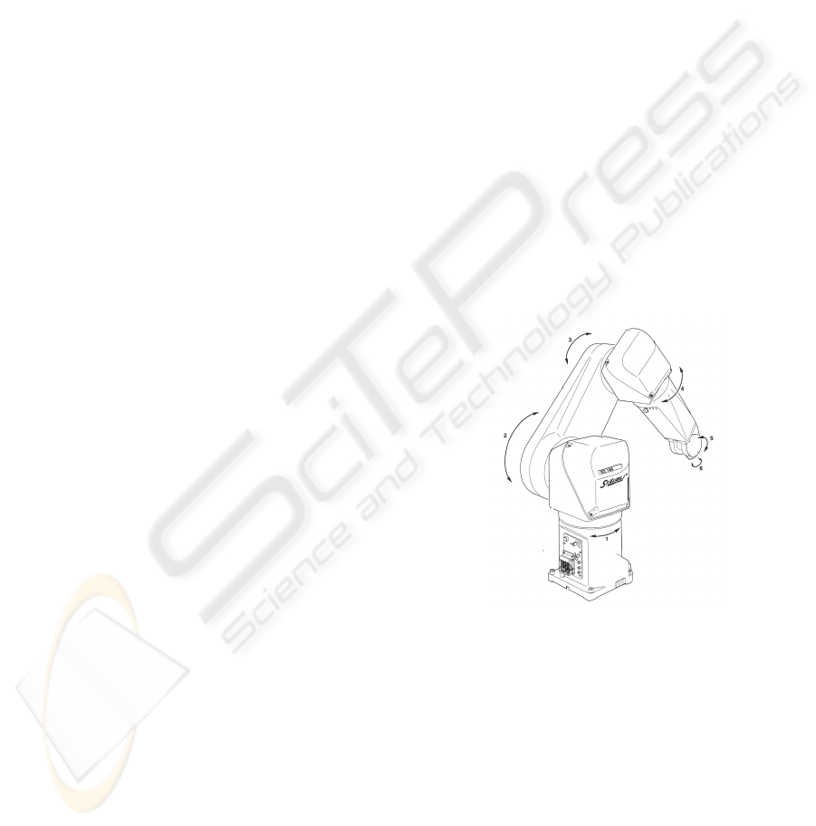
Figure 1: Sketch of the RX130L.

Figure 1 shows a sketchofthe St¨aubli industrial robot.

It is a medium scale robot with six degrees of free-

dom, 1.6 m reach and a total mass of 235 kg.

Fundamentally, the basis for model based control

approaches are the equations of motion

M(q)

q+ G(q,

q+ Q(q,

q) = Q

∈ R

, (1)

where q denotes the vector of minimal coordinates,

respectively the robots joint angles, M(q) is the con-

ﬁguration dependent, positive deﬁnite and symmetric

mass matrix and G(q,

q) contains the velocity depen-

dent nonlinearities as coriolis and centrifugal forces.

The vector Q(q,

q) consists of all generalized forces,

192

Riepl R., Gattringer H. and Bremer H. (2010).

EVALUATION OF FEEDBACK AND FEEDFORWARD LINEARIZATION STRATEGIES FOR AN ARTICULATED ROBOT.

In Proceedings of the 7th International Conference on Informatics in Control, Automation and Robotics, pages 192-197

DOI: 10.5220/0002918301920197

 SciTePress

e.g. forces resulting from gravity or friction. The ac-

tuating motor torques are separated on the right side

of the equations of motion and found in the vector

. The variable n represents the number of degrees

of freedom which equals the number of joints, assum-

ing a rigid multi body system.

The equations of motion, as stated in (1), are com-

monly derived using analytical methods, e.g. with the

Lagrange equations. However, an articulated robot

consists of several joints and may be regarded as an

assembly of n arm/motor units.

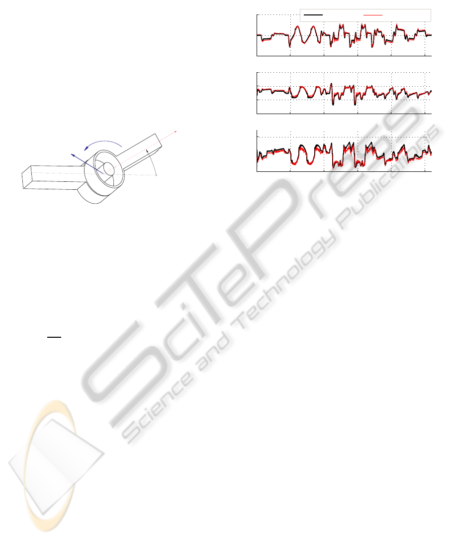
Introducing such a unit, also called subsystem, as

sketched in Figure 2,

Figure 2: An arm/motor subsystem.

with the vector





(2)

containing the translational and rotational velocities

and ω

of the k-th subsystems reference frame and

the corresponding joint angle q, leads with the projec-

tion equation

sub

∑

k=1



∂



+ G

− Q

] = 0 (3)

in subsystem representation, see (Bremer, 2008), to

the equations of motion. This synthetical method,

based on projecting the linear and angular momen-

tum in the free directions of movement, effectively

makes use of the serial composition of several at-

tached arm/motor units. The interested reader may

ﬁnd more information on the subsystems matrices and

vectors, M

, G

and Q

and their detailed derivation

in (Gattringer, 2006).

2.1 Model Veriﬁcation

After an identiﬁcation process as suggested in (Sciav-

icco and Siciliano, 2004; Khalil and Dombre, 2004),

the model parameters are veriﬁed by comparing mea-

sured and simulated motor torques. The simulation

is carried out by integrating the equations of mo-

tion. The reference trajectory for veriﬁcation pur-

poses strictly differs from the ones used during the

identiﬁcation process to assure the parameters’ cor-

rectness in the whole task space.

Figure 3 presents the accordance of the ﬁrst three

joints. Joints four to six are of equivalent quality.

0 5 10 15 20 25

−5

in Nm

Simulation Measurement

0 5 10 15 20 25

−10

−5

in Nm

0 5 10 15 20 25

in Nm

Time in s

Figure 3: Measured versus simulated motor torques.

3 MOTION CONTROL

This section summarizes the control strategies for

tracking the tool center point along a desired trajec-

tory. All introduced methods are part of the evaluation

process.

3.1 Decoupled PD-control

As the name suggests, the decoupled PD-control is

a decentralized single joint control law. Each single

axis compensates the nonlinearities, e.g. inﬂuences

from the other joints, while tracking the desired refer-

ence trajectory in joint space. The control law is given

= K

− q) + K

(

−

q), (4)

where the lower right index d denotes the desired ref-

erence values for joint positions and velocities. The

positive deﬁnite diagonal matrices K

and K

are the

proportional and derivative gains.

The major disadvantage of this common and sim-

ple control law is the lack of knowledge about the sys-

tem which is to be controlled.

Asymptotic stability can only be proven if the sys-

tem remains in steady state with the classical stabil-

ity theorems of mechanical systems, summarized in

(Bremer, 1988).

EVALUATION OF FEEDBACK AND FEEDFORWARD LINEARIZATION STRATEGIES FOR AN ARTICULATED

ROBOT

193

3.2 Decoupled PD-control with

Feedforward

To negate the major drawback of the decoupled PD-

control an additional feedforward term is inserted into

control law (4), yielding

= K

− q) + K

(

−

q) + u

. (5)

Effectively exploiting the system knowledge, ob-

tained through the dynamic modeling and identiﬁ-

cation, the necessary reference motor torques which

guide the tool center point along a desired trajectory,

are given with the equations of motion (1) and are so

intuitively suitable for a feedforward control

= M(q

)

+ G(q

)

+ Q(q

). (6)

Obviously, if the reference trajectory is two times

continuously differentiable with respect to time, the

resulting feedforward torques will show a continu-

ous progression. This set of feedforward control is

also called exact feedforward linearization in litera-

ture, see (Hagenmeyer and Delaleau, 2003).

With this choice the PD-controller’s task is re-

duced to compensate modeling inaccuracies, param-

eter variations and external or unknown disturbances.

Proving asymptotic stability, however, still leads

to further challenges, because inserting the feedfor-

ward term and evaluating the equations of motion

transforms the dynamics to a nonlinear time-variant

system. The interested reader may ﬁnd more infor-

mation in (Kugi, 2008; Hagenmeyer and Delaleau,

2003).

3.3 Computed Torque

Introducing the computed torque control law

= M(q)

v+ G(q,

q+ Q(q,

q) (7)

and inserting it into the equations of motion (1) yields

the system

q = v (8)

of n double integrators, resulting in a solely linear in-

terrelation between the new system input v and the

joint angles q. A possible choice for the new system

input v is

v =

+ K

(

−

q) + K

− q) (9)

with the positive deﬁnite diagonal matrices K

and

as stabilizing gains.

By deﬁning the joint tracking error e = q

−q and

inserting Equation (9) in (8) the system dynamics of

the tracking error e for the closed loop system

−

q+ K

(

−

q) + K

− q) = 0

e+ K

e = 0 (10)

is found. Equation (10) instantly allows to shape the

error dynamics by choosing the gains K

and K

, for

example by pole placement.

Please note, in literature the computed torque

method is also referred to as inverse dynamics,

feedback linearization or ﬂatness based control, as

(Isidori, 1985; Slotine and Li, 1990; Fliess et al.,

1995) describe.

3.4 Extended Linearization

Similar to Subsection 3.3, the nonlinearities in the

equations of motion are eliminated with the control

law

= M(q)(

v+ K

q+ K

+ G(q,

q+ Q(q,

q). (11)

Inserting the control law (11) into the equations of

motion (1) yields

q = v− K

q− K

q (12)

or equivalent in state space representation







0 E

−K

 







(13)

which describes the dynamics of the closed loop sys-

tem. Apparently, this MIMO-system is controllable

with the whole repertory of tools available from linear

system theory, for example linear quadratic regulators

or pole placement, well summarized in (Chen, 1998).

Certainly, before designing a linear controller for

system (13), the matrices K

and K

need to be cho-

sen. It is suggested to pick them in a manner so

that the closed loop system (13) resembles its phys-

ical counterpart. One suggestion is that the eigenval-

ues of the linearized equations of motion may be used

as guideline for picking the eigenvalues of the closed

loop system. However, due to stability issues positive

eigenvalues in the closed loop system (13) need to be

avoided.

Asymptotic stability of Equation (13) is derived

with linear system theory.

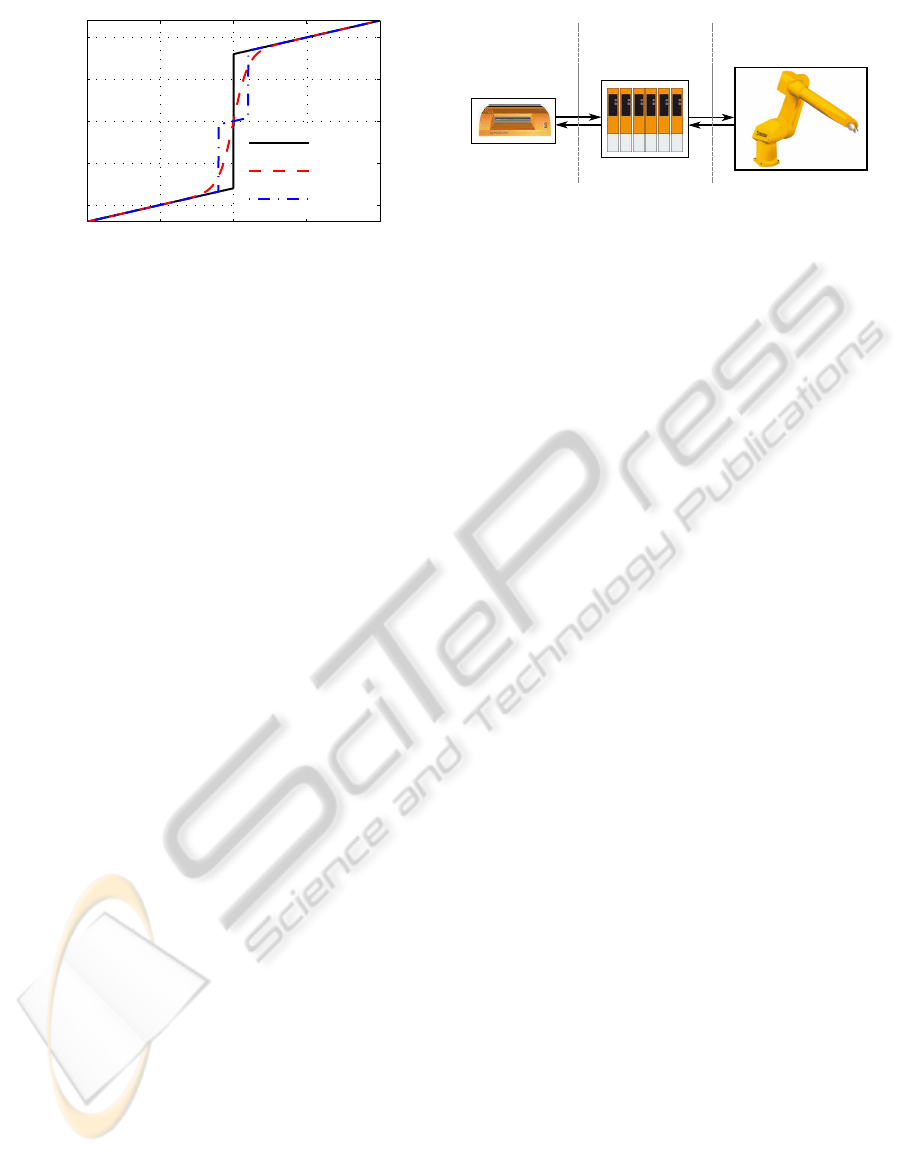
3.5 Friction Feedback Issues

One common problem with feedback linearization

methods occurs when friction models are part of the

inverse dynamics. This is usually the case for any me-

chanical or robotic application. If the classical model

for friction

fric

= d

˙q+ d

signum ( ˙q) (14)

is part of the feedback loop, then the noisy measure-

ment of the velocity signal ˙q will be ampliﬁed and fed

ICINCO 2010 - 7th International Conference on Informatics in Control, Automation and Robotics

194

−1−2

−5

−10

Joint velocity ˙q

Friction Torque

fric

fric,b

fric,a

Figure 4: Friction models for feedback loop.

through to the actuators, directly resulting in a dis-

turbing hum.

To counter this effect the friction characteristics

in the feedback loop have to be adapted. Two simple

solutions are given by

fric,a

= d

˙q+ d

signum ( ˙q) for ˙q ≥ ε

fric,a

= 0 else

fric,b

= d

˙q+ d

tanh ( ˙q/ε

)

(15)

with suitable values for ε

and ε

. Figure 4 shows the

original and adapted friction models.

4 EXPERIMENTS

The introducedcontrol strategies are evaluated in a se-

ries of experiments. Additionally, details on the labo-

ratory setup and the recorded data are the dominating

topics of this section.

4.1 Setup

In the laboratory, the St¨aubli RX130 industrial robot

is interfaced with state-of-the-art motion hardware.

All mechanical and electrical parts of the robot itself,

like motors and resolvers, remain untouched. The

servo drives, powering the synchronous motors, and

the digital processing unit are of industrial standard

but still offer the necessary development tools for im-

plementing the proposed methods.

Figure 5 shows the main components and their in-

terrelation to each other. The central computing unit

is connected to six servo drives via a high-speed Pow-

erlink bus. Each servo drive acts as an ampliﬁer for

the AC motor, evaluates resolver signals and may use

an internal linear cascaded controller for position and

velocity control of the attached motors.

Automation

Servo

Drives

Robot Mechanics

Figure 5: Setup.

4.2 Trajectory

A reference trajectory with signiﬁcant characteristics

is necessary for the process of evaluation. It needs to

cover a reasonable workspace while containing high

dynamics, even in disadvantageous poses and conﬁg-

urations.

A suitable choice, meeting this prerequisites, is

found in (ISO NORM 9283, 1998) which originally

deﬁnes a standardized trajectory for tool center point

measurements and evaluations. By sharing a common

objective, the proposed trajectory is also the reference

in the following experiments.

The velocity and acceleration of the tool center

point is given with 1 m/s and 5 m/s

. These set-

tings represent the highest values without exceeding

the available actuating torques. The trajectory itself is

a composition of straight lines, circles and squares in

space.

The inverse kinematics is computed numerically,

yielding the according joint values and their deriva-

tives with respect to time. It is also guaranteed that

all reference joint angles are two times continuously

differentiable with respect to time.

4.3 Centralized / Decentralized Control

When realizing the introduced control structures on

the industrial hardware, the feedforward and feed-

back approach show major differences. Basically, the

model based control methods – feedforward as well

as feedback – evaluate the equations of motion each

sample step in order to linearize the mechanical sys-

tem. Furthermore some stabilizing gains guarantee

stability.

However, in the case of feedforward control,

which is a decoupled and decentralized method, the

stabilizing PD feedback loop may be implemented di-

rectly on the servo drives which proﬁt from very short

response times and a fast sampling rate. On the other

hand, linearizing the system only by using reference

values instead of actual ones, is not as exact as with

feedback linearization.

EVALUATION OF FEEDBACK AND FEEDFORWARD LINEARIZATION STRATEGIES FOR AN ARTICULATED

ROBOT

195

x 10

−5

−1

−3

0.01

−0.01

in rad

time t in s

Lin

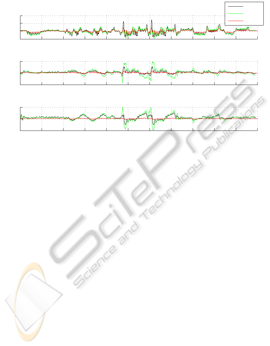
Figure 6: Lag errors with various control strategies.

4.4 Results

During a series of experiments the lag errors of the

joints are recorded. Due to the rigid construction and

the high stiffness of the gears, the joints’ lag errors

may be used to give estimations for the tool center ac-

curacy. Also, all design parameters are chosen with

highest possible gains which were evaluated in an-

other set of preceding investigations.

In Figure 6, the lag errors for joint one, two and

three are revealed. The lag errors resulting with ex-

tended linearization are denoted with e

Lin

, respec-

tively the ones with computed torque and feedforward

with e

and e

While the performance of the control methods

seems to be nearly equal for joint one, the joints

two and three show different results. Especially axes

with high loads resulting from gravity are beneﬁting

from their reduced lag errors with the feedforward ap-

proach.

The axes four, ﬁve and six are of similar behav-

ior and thus omitted. All values presented are joint

angles, transformed to the gears’ output sides.

5 INTERPRETATION

It is clearly not immediately evident that the feedfor-

ward linearization excels in performance in case of

this robotic application. The reason lies in the struc-

ture of control. If the feedforward linearization

is used in combination with the decoupled PD - con-

trol, the servo drives assume the task of decentralized

controllers. These decentralized controllers proﬁt

from very short cycle times, still supported by the

feedforward variables.

The centralized control methods, which linearize

the system by feedback, are mathematically outstand-

ing and superior. However, due to the delays which

arise from closing the feedback loop to the central

processing unit, the maximum gains are drastically re-

duced. Thus, deviations from the model and external

disturbances are eliminated in a slower manner.

The effort for preparation – originating from ob-

taining the dynamic model with a valid and well iden-

tiﬁed set of parameters – is equal for all proposed

model-based control strategies because they share a

common origin, the equations of motion.

To sum up, the method of choice to control the

motion of an articulated robot with six axes is the

feedforwardlinearization approach. Model based sys-

tem knowledge can effectivelybe exploited to support

the servo drives internal, fast sampling controllers

which are technically mature and professional prod-

ucts.

6 CONCLUSIONS

With the interpretation at hand, the feed forward lin-

earization technique is investigated in more detail.

From a practical viewpoint, the endeffector error

ICINCO 2010 - 7th International Conference on Informatics in Control, Automation and Robotics

196

along a given trajectory is a characteristic of interest.

Assuming a rigid model and high gear stiffnesses, the

forward kinematics is evaluated to compute the de-

viation between the desired trajectory and the actual

trajectory.

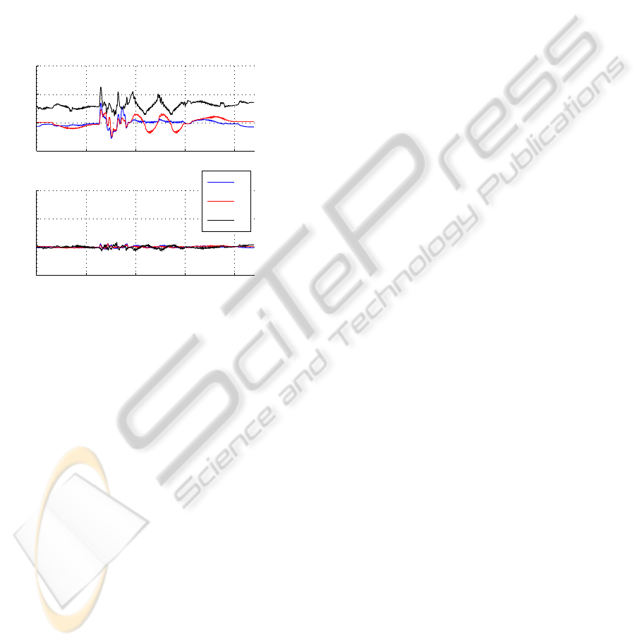
To analyze the effects of the feedforward lin-

earization, the experiment is conducted with and

without superimposed feed forward loop. Figure 7

shows the tool center point (short TCP) error in iner-

tial coordinates. The x- and y-axes are parallel to the

robots mounting surface whereas the z-axis points in

the same direction as the gravity vector.

0 5 10 15 20

−5

x 10

−3

TCP error in m

without feed−forward

0 5 10 15 20

−5

x 10

−3

Time in s

TCP error in m

with feed−forward

Figure 7: Evolution of TCP errors.

Interpreting the plot shows, that the robots manip-

ulator has nearly an average of 4 mm deviation in di-

rection of the z-axis. This static payload of the robot’s

own mass is instantly compensated with the feed for-

ward approach. During the phases with high dynam-

ics, the result with feed-forward control is also con-

siderably improved.

ACKNOWLEDGEMENTS

The authors acknowledge the support and coopera-

tion with Bernecker & Rainer, especially the group

of Alois Holzleitner and Gernot Bachler. The motion

control system provided allows quick implementation

and offers technical perfection which made this re-

search possible.

REFERENCES

Bremer, H. (1988). Dynamik und Regelung mechanischer

Systeme. Teubner Studienb¨ucher, Stuttgart.

Bremer, H. (2008). Elastic Multibody Dynamics: A Di-

rect Ritz Approach, volume 35 of Intelligent Systems,

Control, and Automation: Science and Engineering.

Springer-Verlag GmbH.

Chen, C.-T. (1998). Linear System Theory and Design (Ox-

ford Series in Electrical and Computer Engineering).

Oxford University Press, third. edition.

Fliess, M., L´evine, J., and Rouchon, P. (1995). Flatness and

defect of nonlinear systems: Introductory theory and

examples. International Journal of Control, 61:1327–

1361.

Gattringer, H. (2006). Realisierung, Modellbildung und

Regelung einer zweibeinigen Laufmaschine. PhD the-

sis, Johannes Kepler Universit¨at Linz.

Hagenmeyer, V. and Delaleau, E. (2003). Robustness anal-

ysis of exact feedforward linearization based on dif-

ferential ﬂatness. Automatica, 39(11):1941 – 1946.

Isidori, A. (1985). Nonlinear Control Systems. Springer-

Verlag.

ISO NORM 9283 (1998). Manipulating industrial robots -

performance and criteria. Norm, EN ISO 9283.

Khalil, W. and Dombre, E. (2004). Modeling, Identiﬁcation

and Control of Robots. Kogan Page Science, London.

Kugi, A. (2008). Introduction to tracking control of ﬁnite-

and inﬁnite-dimensional systems. Stability. Identiﬁ-

cation and Control in Nonlinear Structural Dynamics

(SICON).

Sciavicco, L. and Siciliano, B. (2004). Modelling and Con-

trol of Robot Manipulators. Springer, United King-

dom.

Slotine, J.-J. and Li, W. (1990). Applied Nonlinear Control.

Prentice Hall.

EVALUATION OF FEEDBACK AND FEEDFORWARD LINEARIZATION STRATEGIES FOR AN ARTICULATED

ROBOT

197