EXPERIMENTS WITH A CONTINUUM ROBOT STRUCTURE

Dorian Cojocaru, Sorin Dumitru, Florin Manta, Giuseppe Boccolato

Faculty of Automation, Computers and Electronic, University of Craiova, Bld. Decebal, Craiova, Romania

Ion Manea

Faculty of Mechanics, University of Craiova, Calea Bucuresti Str., Craiova, Romania

Keywords: Continuum Robots, Kinematics, Mechanical Experiments.

Abstract: A continuum arm prototype was designed and implemented using two different shapes: cylinder like and

cone like. This new robot is actuated by stepper motors. The rotation of these motors rotates the cables

which by correlated screwing and unscrewing of their ends determine their shortening or prolonging, and by

consequence, the tentacle curvature. The kinematics and dynamics models, as well as the different control

methods developed by the research group were tested on these robots. The lack of no discrete joints is a

serious and difficult issue in the determination of the robot’s shape. A solution for this problem is the vision

based control of the robot, kinematics and dynamics. An image – based visual servo control where the error

control signal is defined directly in terms of image feature parameters was designed and implemented. In

this paper, we analyze some mechanical capabilities of this type of continuous robots. We present the

structure of the tentacle robot, it’s kinematics model and the results for a series of tests regarding the

mechanical behaviour of the robotic structure.

1 INTRODUCTION

Modern industrial robots are mostly (human) arm-

inspired mechanisms with serially arranged discrete

links. When it comes to industrial environment

where the workspace is structured and predefined

this kind of structure is fine. This type of robots are

placed in carefully controlled environments and kept

away from human and their world.

When it comes to robots that must interact with

the natural world, it needs to be able to solve the

same problems that animals do. The rigid structure

of traditional robots limit their ability to maneuver

and in small spaces and congested environments,

and to adapt to variations in their environmental

contact conditions (Suzumori et al., 1991),

(Robinson and Davies, 1999). For improving the

adaptability and versatility of robots, recently there

has been interest and research in “soft” robots

(Cowan and Walker, 2008). In particular, several

research groups are investigating robots based on

continuous body “continuum” structure. If a robot’s

body is soft and/or continuously bendable it might

emulate a snake or an eel with an undulating

locomotion (Crespi and Ijspeert, 2006).

The continuum or hyper-redundant robot

manipulators behaviour is similar to biological

trunks, tentacles or snakes. The movement of the

continuum robot mechanisms is generated by ending

continuously along their length to produce a

sequence of smooth curves (Blessing and Walker,

2004). This contrasts with discrete robot devices,

which generate movement at independent joints

separated by supporting links.

We can also describe as continuum robots snake-

like robots and elephant’s trunk robots, although

these descriptions are restrictive in their definitions

and cannot be applied to all snake-arm robots. A

continuum robot is a continuously curving

manipulator, much like the arm of an octopus

(Davies, J.B.C., 1998). An elephant’s trunk robot is

a good descriptor of a continuum robot. The

elephant’s trunk robot has been generally associated

with an arm manipulation – an entire arm used to

grasp and manipulate objects, the same way that an

elephant would pick up an apple. Snake-arm robots

are often used in association with another device

meant to introduce the snake-arm into the confined

space. However, the development of high-

198

Cojocaru D., Dumitru S., Manta F., Boccolato G. and Manea I. (2010).

EXPERIMENTS WITH A CONTINUUM ROBOT STRUCTURE.

In Proceedings of the 7th International Conference on Informatics in Control, Automation and Robotics, pages 198-205

DOI: 10.5220/0002921501980205

 SciTePress

performance control algorithms for these

manipulators is quite a challenge, due to their unique

design and the high degree of uncertainty in their

dynamic models. The great number of parameters,

theoretically an infinite one, makes very difficult the

use of classical control and the conventional

transducers for position and orientation.

2 THE ROBOTIC STRUCTURE

A research group from the Faculty of Automation,

Computers and Electronics, University of Craiova,

Romania, started working in research field of hyper

redundant robots over 20 years ago. The

experiments started on a family of TEROB robots

which used cables and DC motors. The kinematics

and dynamics models, as well as the different

control methods developed by the research group

were tested on these robots. Since 2008, the research

group designed a new experimental platform for

hyper redundant robots.

Our robotic system is composed from two units,

one with a flexible structure with kinematic

possibilities similar with the snake’s locomotion and

another one with driving. The flexible unit is

composed from three modules with independent

driving, that confers a complex 3D configuration,

with multiple kinematic possibilities for the working

space. The flexible structure is conceived in modular

systems with decoupling possibilities for a

controlled optimization of the working space.

The flexible structure as an integrate system, or

as independent modules, is conceived to allow

driving in two modes, respective:

- one with wires and a flexible central column;

- one with flexible vertebrates and a flexible

central column;

In the case where the driving is made by wires, a

module has two freedom degrees and in the case of

driving with flexible columns each module has three

degrees of freedom. As it can be observed the

flexible unit structured in three modules for

controlling a complex workspace, with multiple

kinematic possibilities. The machine structure for

each module is based upon thread transmissions with

self decelerations possibilities and adjust of the

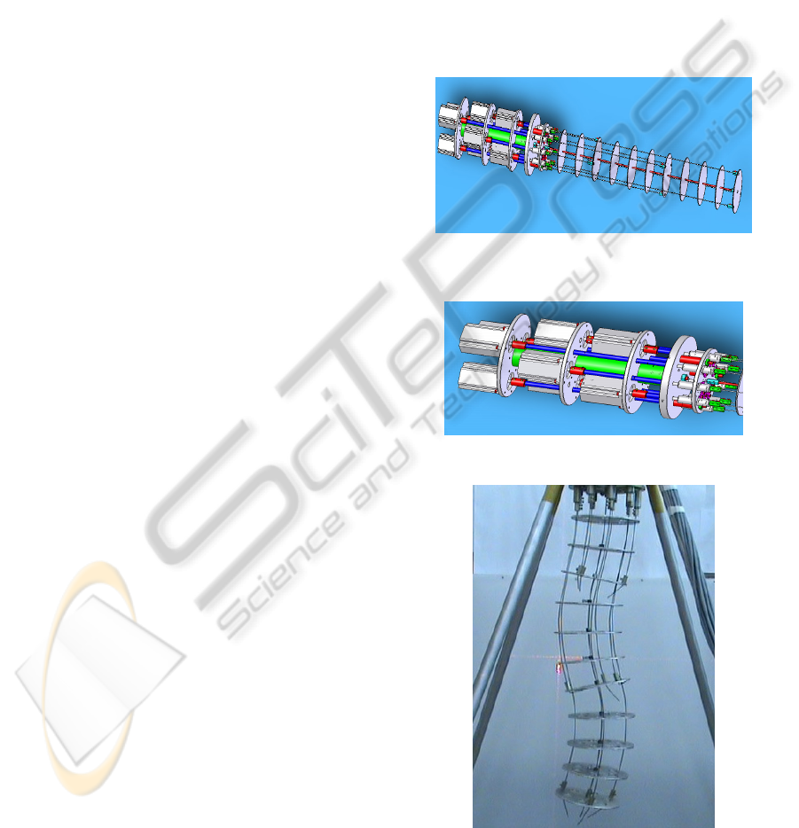
axial-radial clearances.The flexible unit with the

snake-like design is composed from a base flange,

some intermediary flanges, and four flexible shafts,

with high elasticity, which will be called vertebral

spines. The central shaft is mounted rigidly to all the

intermediary flanges, fig. 1.

The three super elastic spines are mounted

equidistantly upon the central spine. The entire

vertebrates are connected only to the end flange. The

intermediary flanges maintain constant the radial

distance between the secondary tubes and the central

vertebrate. Changing in an active way the length for

two of the vertebrate spines, the final flange can be

manipulated with two degrees of freedom in any

direction.

The three actuating spines are rigidly jointed

only to the end flange, the joint between them and

the intermediary flanges is like one translational

joint.

Figure 1: The virtual model with the driving and vertebral

unit.

Figure 2: Redundant driving unit.

Figure 3: The assembly of the robotic system with the

baggy vertebral unit.

EXPERIMENTS WITH A CONTINUUM ROBOT STRUCTURE

199

2.1 Experimental Modelling

As it was presented above, the robot is designed in a

modular structure, with three modules,

independently actuated through thread transmissions

with possibility to adjust the radial and axial

clearances, in the aim to assure the imposed

kinematics precision. The vertebrate unit is designed

to work in two ways, respectively with two or three

degrees of freedom on each module.

2.2 Modelling with Finite Elements

For demonstrating the viability of mechanical

system it is proposed the modelling and simulation

functionality with finite element method. Faithfully

are respected the shape conditions and loadings, so

that through a Virtual Prototyping attempt it is

obtained a parameterized virtual system, which can

be loaded so that you get various types of deformed

shapes, obviously controlled for the analyzed

mechanic system (Dumitru et al., 2009).

Parameterized modelling of the flexible system

allows 3D simulation for different variants with one,

two or three modules, with different size dimensions

and types of materials with circular vertebras full or

tubular, in this way assuring a wider area of skills

for the proposed and analyzed system.

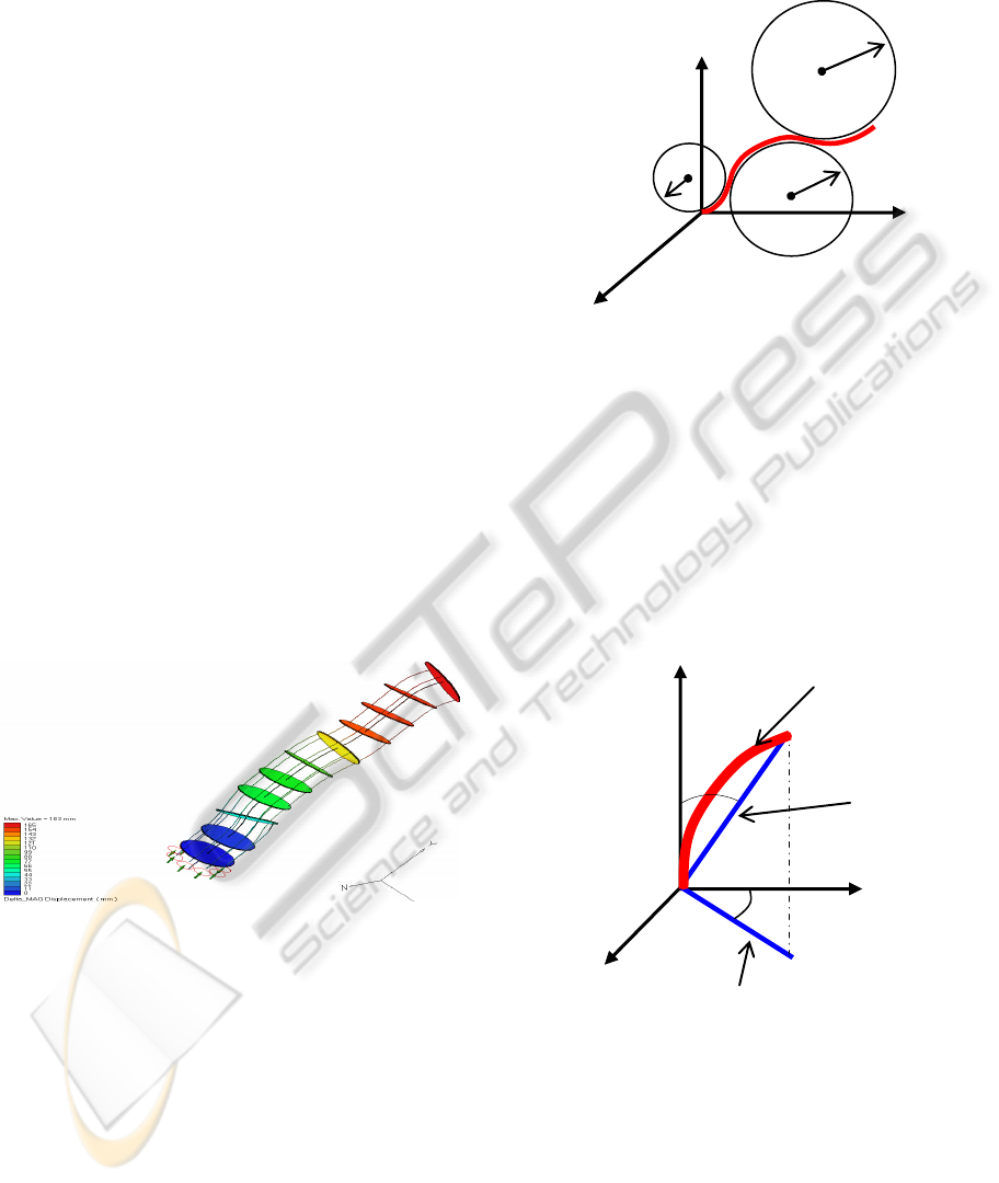
Figure 4: Elastic displacement distribution for a kinematic

chain with 3 modules.

3 THE KINEMATIC MODEL OF

THE TENTACLE ARM

In order to control a hyper-redundant robot we have

to develop a method to compute the positions for

each one of his segments (Ivanescu et al., 2006). By

consequence, given a desired curvature S*(x, tf) as

sequence of semi circles, identify how to move the

structure, to obtain s(x, t) such that:

),(),(lim

ftt

txStxs

→

(1)

where x is the column vector of the shape

description and tf is the final time (see Fig. 6).

X

2

1

Z

Figure 5: The description of the desired shape.

3.1 Tentacle Shape Description

The tentacle’s shape will be described considering

two angles (θ, α) for each segment, where θ is the

rotation angle around Z-axis and is the rotation angle

around the Y-axis (see Figure 5). In order to

describe the movement we can use the roto-

translation matrix as shown in Figure 6. Figure 7

shows the relation between the orientation of one

projection on the main plane segment and the

curvature angle of the previous segment.

X

Y

Z

segment

chord

projectiononthemainplane

Figure 6: The description of a 3D curvature.

(

)

(

)

() ()

⎥

⎦

⎤

⎢

⎣

⎡

⋅

⋅⋅

⋅

⋅⋅

−

100

)cos(L

cos

sin

)sin(L

sin

cos

ββ

(2)

The generic matrix in 2D that expresses the

coordinate of the next segment related to the

previous reference system can be

written as follow:

ICINCO 2010 - 7th International Conference on Informatics in Control, Automation and Robotics

200



centre

originalpositionofthe

segment

L

2β

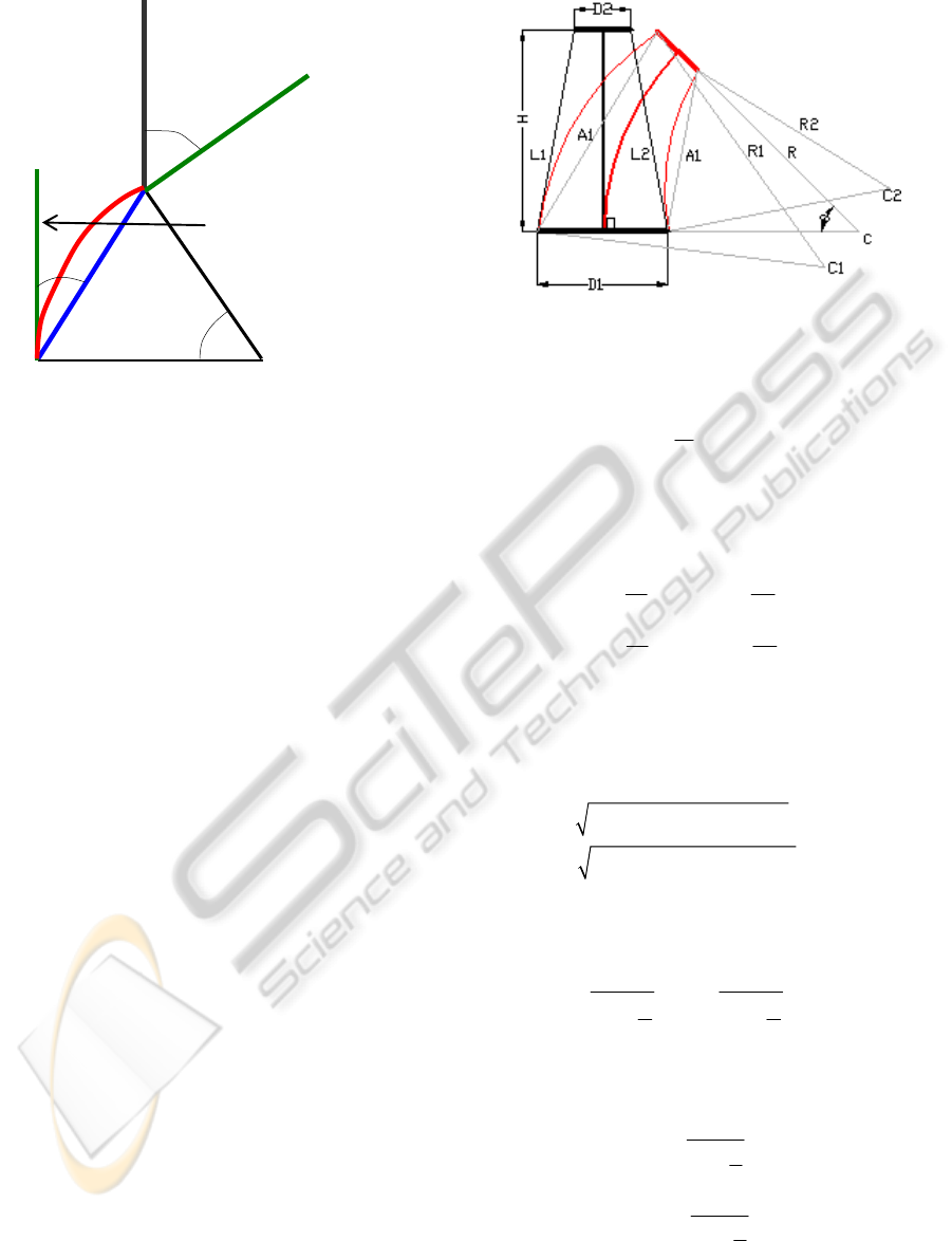
Figure 7: Curvature and relation between θ

and β.

In 3D space we cannot write immediately the

dependence that exists between segments. This

relation can be obtained through the pre-

multiplication of generic roto-translation matrix

(Cojocaru et al., 2008). One of the possible

combinations to express the coordinate of the next

segment related to the frame coordinate of the

previous segment is the following:

:()()()()

iiiiiiii

generic z y y z

RRTrVRR

αθ

=⋅ ⋅⋅

(3)

where

)(R

and

)(R

are the fundamental

roto-translation matrix having 4x4 elements in 3-D

space, and Try(V) is a 4x4 elements matrix of pure

translation in 3-D space and where Vi is the vector

describing the translation between two segments

expressed in coordinate of i-th reference system. The

main problem remains to obtain an imposed shape

for the tentacle arm. In order to control the robot, we

need to obtain the relation between the position of

the wires and the position of the segment.

3.2 Curvature of One Segment

In the current stage of our research, a decoupled

approach is used for the robot control scheme, thus

the three segments are

controlled separately, without

considering the interaction between them. This

section presents the way direct kinematics of one

segment was obtained. The geometry of one

segment for the 2D case is described in Fig. 10. The

curvature angle θ of the segment is considered as the

input parameter, while the lengths L1 and L2 of the

control wires are the outputs (Boccolato et all.,

2009).

Figure 8: The geometry of one segment.

The radius R of the segment curvature is

obtained using equation (4):

(4)

where H is the height of the segment. The following

lengths are obtained from Fig. 10, based on the

segment curvature:

11 12

21 22

LR LR

=+ =+

=− =−

(5)

where D1 and D2 are the diameters of the segment

end discs.

Based on the Carnot theorem, the lengths A1 and A2

are then obtained:

22 22

11112 1112

22 22

22122 2122

2cos

ALL LL

=+−⋅⋅⋅

(6)

The control wires curvature radius R1 and R2 are

given by the relations (7):

2 sin 2 sin

⋅⋅

(7)

Finally, the lengths of the control wires are

obtained as in (8):

2sin

⋅

=⋅=

⋅

=⋅=

⋅

(8)

EXPERIMENTS WITH A CONTINUUM ROBOT STRUCTURE

201

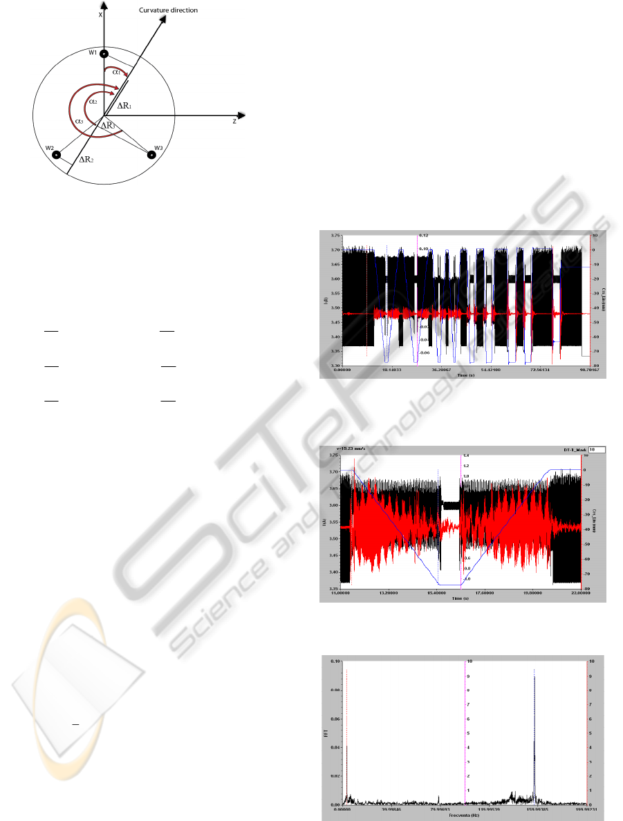
Figure 9: Projection of the wire to get the

direction.

For the 3D case, a virtual wire is considered,

which gives the α direction of the curvature.

Considering one virtual wire in the direction of the

desired curvature having length calculated as below.

First, the following lengths are calculated:

)cos(

RL)cos(

)cos(

RL)cos(

)cos(

RL)cos(

223

222

121

αα

⋅+=⋅+=

(9)

⎪

⎩

⎪

⎨

⎧

−°=

−=

αα

240

120

(10)

Based on (6) and (9) the curvature radius R1, R2

and R3 of the three control wires are then obtained.

Finally the lengths of the control wires are

calculated with relation (11):

⋅=

⋅

33w

22w

11w

(11)

Besides, for the system presented we can obtain

two useful relations:

cos( ) 0

⎧

⎪

⎨

⎪

⎩

∑

(12)

The second equation can be utilized to estimate

the compression or the extension of the central bone.

4 EXPERIMENTS

We conducted a series of experiments, having as

purpose the analysis of the robotic structure,

including the behavior of the arm and the stepper

motors used for its actuation.

For these tests, we used the following equipment:

 Spider 8 acquisition system, with eight input

channels and 12 bit resolution per channel

 Nexus 2692-A-0I4 signal conditioner with load

compensation, four input/output channels,

frequency domain 0.1Hz ÷ 100KHz and linear-

ity error ≤0.05%;

 Bruel&Kjaer model 4391 accelerometers,

frequency domain 0.3 ÷ 10000Hz, load 1 pC/ms-

2, linearity error ≤1%;

Figure 10: Recorded dataset. Marked with black - the

current, with red - end effector oscillation and with blue -

the displacement.

Figure 11: Recorded data for a movement executed at

19.23 mm/s.

Figure 12: Frequency analysis for oscillation. Slow speed

case.

ICINCO 2010 - 7th International Conference on Informatics in Control, Automation and Robotics

202

 WA300 inductive transducer for linear

displacement, displacement range 0÷300mm,

linearity error ≤1%;

 MicroSwitch model CSLA 20KI current

transducer, current domain ±20A, linearity

error ≤1%

 The data was recorded on a IBM notebook with

Testpoint V5.1 soft-ware installed

We placed the sensors as follows:

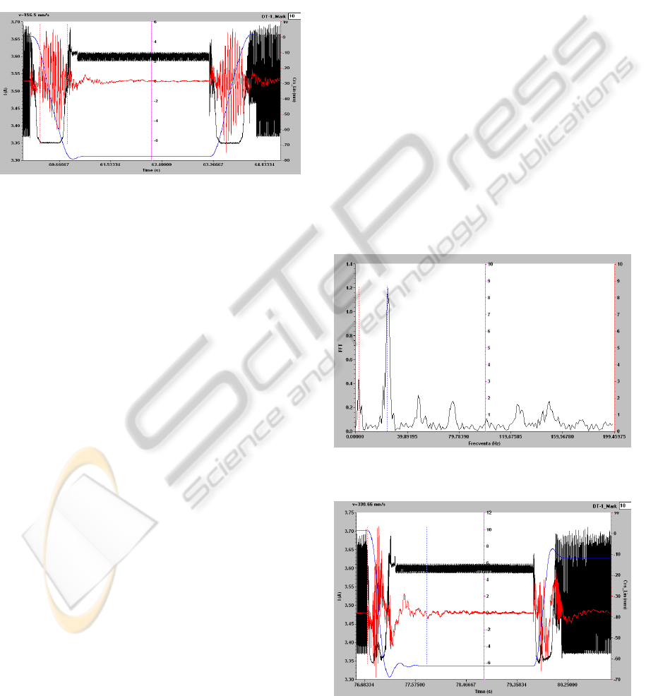
Figure 13: Medium speed movement (156.99 mm/s).

 The displacement sensor was connected at the

robot’s arm free end. The objective is to

measure the total displacement realized by the

end effector. Because of the sensor’s intrinsic

structure, and for obtaining a linear relation

between sensor measurement and robot

displacement in the 3D space, we restricted the

robot’s movement to a movement in a plane

formed by the robot’s backbone and the

sensor’s extension axis

 The accelerometer was placed in the same

point as the displacement sensor. The objective

is to determine the vibration induced in the

robot arm structure by the actuation system and

the control algorithm.

 The ammeter was connected in a serial mode

with one of the stepper motor phases (the

stepper motors are tree phases ones). The

objective is to determine the stepper motor

current need during the movements, and also to

detect if and when the losing steps

phenomenon occurs, based on the fact that a

losing step process can be noticed by observing

a high current peak.

In the figure 10 can be observed a recorded

dataset. The measured current is represented with

black color, with blue is represented the arm

displacement, and with red is marked the oscillation

recorded at the end of the robot arm. The dataset

recorded a same trajectory described by the robot,

but at different speeds. In the left side can be

observed the movement execution at a lowest speed

(19.23 mm/s), and in the right side at high speed

(330 mm/s). In the following paragraphs we will

analyze the robot’s behavior for these two extreme

movements. The first move observed was executed

with a speed of 19.23 mm/s, going forward from the

origin to the end point and, after a short break, back

to the original. The detailed recorded data can be

seen in the Figure 11.

The oscillation was amplified 100 times, for

having a better view for its evolution. As expected

for slow moves case, when the effort needed for

robot arm displacement is low, the current evolution

indicates that the stepper motor doesn’t lose any

steps and the movement there is no position error.

Regarding oscillation, one can observe that near the

origin position the robot exhibits a higher oscillation

of its end effector. We consider that this

phenomenon appeared due to the fact that near

origin the tension in the actuation cables is lower,

because the potential energy due gravity have the

lowest value, and at end point the potential energy

have a considerable higher value, conducting to a

higher tension in cables which prevents the robot

arm to oscillate.

Figure 14: Frequency analysis for oscillation. Medium

speed case.

Figure 15: High speed movement.

EXPERIMENTS WITH A CONTINUUM ROBOT STRUCTURE

203

If we take a closer look at the oscillation, and

make a frequency analysis (figure 12), it can be

observed that there are two spikes in frequency, one

at 2.9 Hz, and one at 159.99 Hz.

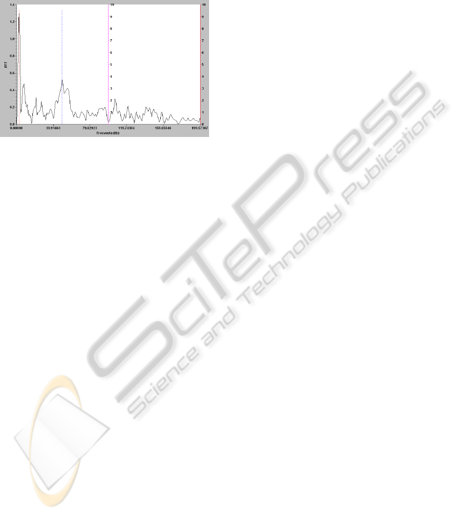
Figure 16: Frequency analysis for oscillation. High speed

case.

As already identified, where an artificial vision

system was used (Tanasie et al., 2009), the first

spike at 2.9 Hz represents the natural resonance

frequency for the robotic arm. By observing the

oscillation analysis for faster movements, we

determined that the second spike, with a higher

level, placed at 159.99 Hz, is induced by the

actuation system – the vibrations frequency

generated by the actuation system and transmitted in

the cables, also being responsible for the resonance

spike at 2.9 Hz.

Considering a medium speed movement (156.99

mm/s), the following dataset was recorded (Figure

13). Analyzing the current evolution, a singular

spike can be observed at 63.8 second on the

timescale, which indicates that the motor loses a

single step, this situation being caused by the fast

stop of the robotic arm. Correlated with this fact, the

analysis of the trajectory evolution shows that the

end of the robot arm don’t stop directly at the

desired position, and under the effect of inertia

determined by its own mass it passes that position.

While the cables exhibit neither compression nor

extension, the position error is determined

exclusively by a shear effect. Shear is an elastic

deformation, thus generating a force that brings the

robot arm back at the desired position. This

transitory effect takes 0.2 seconds and the maximum

position error is 2 millimeters.

The oscillation graph shows a similar evolution

as described for the previous case, but the frequency

analysis gives a different characteristic (Figure 14).

The natural oscillation frequency can be identified as

a spike at the same frequency 2.9 Hz, but the

vibration induced by the actuation system may be

found now at 24.6 Hz, as a result of the motor’s

speed variation.

The last observed evolution is for high speed

movement (330 mm/s). The recorded data is

represented in the Figure 15. The current evolution

is more dramatic and irregular, as can be observed in

the figure 15 (marked with black line). The current

profile isn’t anymore smooth, as in previous cases,

and some major fluctuations can be seen at 76.9 sec

and at 79.7 sec. Those fluctuations correspond to a

large number of lost steps, the effort required for

moving the robot being very large. This conclusion

is sustained by the conclusions of analysis conducted

for displacement and vibration. Regarding the

displacement, the robot was programmed to execute

the very same movement, going from origin to a

desired position and then back to the origin, but at

different speeds. This means that in all recorded

data, the robot must achieve the same desired

position, and the position at the end of the

movement must be the same with the position from

where the movement started (the origin). Observing

the displacement from figure 15 (marked with blue

line), it can be determined a difference of 12 mm

between the beginning position and final position.

Also, if one compares the desired position achieved

in figure 11, 13 and 15, can determine that the

desired position is achieved successfully in figure 11

and 13, but in figure 15 the robot fails to reach the

desired position, introducing a position error of 6

mm. The inertial effect is very high, the robot

presenting a large oscillation before remaining

steady in the desired position. Previous conclusions

are also sustained by the recorded vibrations,

marked with red line in figure 15. On the same

timeline with the current fluctuations can be noticed

a large amplitude of the vibration, as an effect of the

discontinuity in movement determined by lost steps.

Moreover, as the frequency analysis shown in the

figure 16 denotes, this high speed actuation

determines a resonance with the natural frequency of

the robot arm, affecting the robot arm evolution.

5 CONCLUSIONS

As conclusions, for the slow speed moves, there are

no lost steps in stepper motors, meaning that an open

loop control can be successfully applied to the

system. There is a low amplitude oscillation of the

robot’s arm, mainly at 159.99 Hz, induced by the

actuation system, but it induces only a small

ICINCO 2010 - 7th International Conference on Informatics in Control, Automation and Robotics

204

amplitude natural frequency resonance, so the robot

arm doesn’t resonate with actuation system. Also,

considering the displacement (marked with blue in

the figure), it can be observed that the position error

is zero. The overall behavior of the structure is a

very good one.

For the medium speed moves, the stepper motors

may lose steps, but this phenomenon occurs

occasionally and can be considered insignificant if is

evaluated as a ratio lost steps / total number of steps,

meaning that an open loop control can still be

successfully applied to the system. There is a low

amplitude oscillation of the robot’s arm, mainly at

24.6 Hz, induced by the actuation system, but it

induces only a small amplitude natural frequency

resonance, so the robot arm doesn’t resonate with

actuation system. The displacement record reveals a

transient evolution around the final position,

introducing a transient position error, having 2 mm

maximum amplitude and with a short duration, 0.2

seconds. At the end of the transient evolution, the

robot stops on the desired position and the position

error is zero. The overall behavior of the structure is

a good one.

ACKNOWLEDGEMENTS

The research presented in this paper was supported

by the Romanian National University Research

Council CNCSIS through the IDEI Research Grant

ID93 and by FP6 MARTN through FREESUBNET

Project no. 36186.

REFERENCES

Blessing, M., Walker, I. D., 2004. Novel Continuum

Robots with Variable- Length Sections, Proceedings

3rd IFAC Symposium on Mechatronic Systems,

Sydney, Australia, September 2004, pp. 55-60.

Boccolato, G., Manta, F., Dumitru, S., Cojocaru, D., 2009.

3D Control for a Tentacle Robot, 3rd International

Conference on Applied Mathematics, Simulation,

Modelling (ASM'09), Vouliagmeni Beach, Athens,

Greece.

Cojocaru, D., Tanasie, R. T., Marghitu, D. B., 2008. A

Complex Mathematical Expression Operations Tool,

Annals of The Univ. of Craiova, Series: Automation,

Computers, Electronics And Mechatronics, ISSN:

1841-0626, Volume 5(32), no. 1, pp. 7-12.

Cowan, L. S. and Walker, I. D., 2008. “Soft” Continuum

Robots: the Interaction of Continuous and Discrete

Elements, Artificial Life XI.

Crespi, A. and Ijspeert, A. J., 2006. An amphibious snake

robot that crawls and swims using a central pattern

generator. 9th International Conference on Climbing

and Walking Robots (CLAWAR 2006), pp19-27.

Dumitru, S., Cojocaru, D., Dumitru, N., Ciupitu, I.,

Geonea, I., Dumitru, V., 2009. Finite Element

Modeling of a Polyarticulated Robotic System, Annals

of DAAAM, ISSN 1726-9679, pp 969.

Ivanescu, M., Cojocaru, D., Popescu, N., Popescu, D.,

Tănasie, R.T., 2006. Hyperredundant Robot Control

by Visual Servoing, Studies in Informatics and

Control Journal, Volume 15, Number 1, pp93-102,

ISSN 1220-1766.

Robinson, G., Davies, J. B. C., 1999. Continuum robots—

A state of the art. IEEE International Conference on

Robotics and Automation, pp2849–2854. Detroit, MI.

Suzumori, K., Iikura, S., Tanaka, H., 1991. Development

of Flexible Microactuator and its application to

Robotic Mechanisms, Proceedings of the IEEE

International Conference on Robotics and Automation,

pp. 1622-1627.

Tanasie, R. T., Ivanescu, M., Cojocaru, D., 2009. Camera

Positioning and Orienting for Hyperredundant Robots

Visual Servoing Applications, Journal of Control

Engineering and Applied Informatics, Vol 11, No 1,

p19-26, ISSN 1454-8658.

EXPERIMENTS WITH A CONTINUUM ROBOT STRUCTURE

205