
LEARNING DYNAMIC BAYESIAN NETWORKS
WITH THE TOM4L PROCESS
Ahmad Ahdab and Marc Le Goc
LSIS, UMR CNRS 6168, Université Paul Cézanne, Domaine Universitaire St Jérôme, 13397 Marseille cedex 20, France
Keywords: Machine Learning, Bayesian Network, Stochastic Representation, Data Mining, Knowledge Discovery.
Abstract: This paper addresses the problem of learning a Dynamic Bayesian Network from timed data without prior
knowledge to the system. One of the main problems of learning a Dynamic Bayesian Network is building
and orienting the edges of the network avoiding loops. The problem is more difficult when data are timed.
This paper proposes a new algorithm to learn the structure of a Dynamic Bayesian Network and to orient the
edges from the timed data contained in a given timed data base. This algorithm is based on an adequate
representation of a set of sequences of timed data and uses an information based measure of the relations
between two edges. This algorithm is a part of the Timed Observation Mining for Learning (TOM4L)
process that is based on the Theory of the Timed Observations. The paper illustrates the algorithm with a
theoretical example before presenting the results on an application on the Apache system of the Arcelor-
Mittal Steel Group, a real world knowledge based system that diagnoses a galvanization bath.
1 INTRODUCTION
The theory of Timed Observations is the
mathematical framework that defines a Knowledge
Engineering methodology called the Timed
Observation Modeling for Diagnosis methodology
(TOM4D) (Le Goc, 2008) (Figure 1) and a learning
process called Timed Observation Mining for
Learning (Le Goc, 2006). TOM4D and TOM4L are
defined to discover temporal knowledge about a set
of functions of the continuous time x
i
(t) considered
as a dynamic system X(t)={x
i
(t)} called a process.
According to TOM4D, a model of a process X(t)
is a quadruple <PM(X(t)), SM(X(t)), BM(X(t)),
FM(X(t))>. The Perception Model PM(X(t)) defines
the goals of the process X(t). The Structural Model
SM(X(t)) contains the knowledge about the
components and their organization in structures. The
Behavioral Model BM(X(t)) defines the states and
the state transitions that governs the process
evolution over time. Finally, the Functional Model
FM(X(t)) of the process X(t) defines the
mathematical functions linking the values of the
process variables x
i
(t) of X(t). We propose to
represent the Functional Model FM(X(t)) of a
process as a Bayesian Network.
The problem is then to define the learning
A Priori
Knowledge
Timed Observations
Database
TOM4D
Experts
TOM4L
θ(X, Δ)
PM(X(t))
SM(X(t)) BM(X(t))
FM(X(t))
A Priori
Knowledge
Timed Observations
Database
TOM4D
Experts
TOM4L
θ(X, Δ)
PM(X(t))
SM(X(t)) BM(X(t))
FM(X(t))
Figure 1: Global Structure of the Project.
principles of a Bayesian Network (BN) from a set of
sequences of timed data, without prior knowledge to
the process. Most of the proposed algorithm deals
with un-timed data and faces some difficulties in
orienting the edges of the resulting graph and
building the conditional probability tables. These
two problems are more difficult when data are
timed.
The theory of Timed Observations provides the
tools to solve these two problems: the BJ-Measure
of (Benayadi, 2008) and an adequate representation
of a set of sequences of timed data that is called the
Stochastic Representation (Le Goc, 2005). The BJ-
Measure is an informational measure designed to
evaluates the quantity of information flowing in the
Stochastic Representation of a set of sequences of
353
Ahdab A. and Le Goc M. (2010).
LEARNING DYNAMIC BAYESIAN NETWORKS WITH THE TOM4L PROCESS.
In Proceedings of the 5th International Conference on Software and Data Technologies, pages 353-363
DOI: 10.5220/0002928603530363
Copyright
c
SciTePress

timed data. This representation facilitates also the
building for the CPT tables.
The next section presents a short description of
the state of the art techniques concerning the
learning of Dynamic Bayesian Networks (DBN).
Section 3 introduces the basis of the Stochastic
Representation of TOM4L and the BJ-Measure.
Section 4 describes the learning principles we define
from the properties of the BJ-Measure, the DBN
learning algorithm that we proposes is proposed in
section 5 and an application to a theoretical example
is given in section 6 before showing a real life
application of the algorithm in section 7. Our
conclusions are presented in section 8.
2 RELATED WORKS
A BN is a couple <G, > where G denotes a Direct
Acyclic Graph in which the nodes represent the
variables and the edges represent the dependencies
between the variables (Pearl, 1988), and is the
Conditional Probabilities Tables (CP Tables)
defining the conditional probability between the
values of a variable given the values of the upstream
variables of G. BN learning algorithms aims at
discovering the couple <G, > from a given data
base.
BN learning algorithms fall into two main
categories: “search and scoring” and “dependency
analysis” algorithms. The “search and scoring”
learning algorithms can be used when the knowledge
of the edge orientation between the variables of the
system is given (Cooper, 1992), (Heckerman, 1997).
To avoid this problem, dependency analysis
algorithms uses conditional independence tests
(Cheng, 1997), (Cheesseman, 1995), (Friedman
1998), (Meyrs et al, 1999). But the number of test
exponentially increases the computation time
(Chickering, 1994).
(1)
For example, Cheng’s algorithm (Cheng, 1997) for
learning a BN from data falls in the dependency
analysis category and is representative of most of the
proposed algorithms. It is based on the d-separation
concept of (Pearl, 1988) to infer the structure G of
the Bayesian Network, and the mutual information
to detect conditional independency relations. The
idea is that the mutual information I(X, Y) (eq. 1)
tells when two variables are (1) dependent and (2)
how close their relationship is. The algorithm
computes the mutual information I(X, Y) between all
the pairs of variables (X, Y) producing a list L sorted
in descending order: pairs of higher mutual
information are supposed to be more related than
those having low mutual information values. The
List L is then pruned given an arbitrary value of the
parameter
ε
: each pair (X, Y) so that I(X, Y)< is
eliminated of L. In real world applications, list L
should be as small as possible using the parameter.
This first step (Drafting) creates a structure to start
with but it might miss some edges or it might add
some incorrect edges.
(2)
The second step (Thickening) phase tries to separate
each pair (X, Y) in L using the conditional mutual
information I(X, Y | E) (eq. 2) where E is a set of
nodes that forms a path between the current tested
nodes X and Y from L. When I(X, Y | E)>, then the
edges of the path E should be added between the
current nodes X and Y. This phase continues until the
end of list L is reached. The last step of the
algorithm (Thinning) searchs, for each edge in the
graph, if there are other paths besides this edge
between these two nodes. In that case, the algorithm
removes this edge temporarily and tries to separate
these two nodes using equation (2). If the two nodes
cannot be separated, then the temporarily removed
edge will be returned. After building the DBN
structure, the orientation of the edges and the CP
Tables’ computation is to be done. The procedure
used by (Cheng, 1997) is based on the idea of
searching for the nodes forming a V-Structure
X→Y←Z using the conditional mutual information,
and then trying to deduce the other edges from the
discovered one. This procedure have a very big
limitation which is that if a network does not contain
a V-Structure, no edge can be oriented.
The two main limitations of the methods of the
dependency analysis category are so the need of
defining the parameter and the exponential amount
of Conditional Independence tests to orient the edges
of the graph.
3 TOM4L FRAMEWORK
The Timed Observation Mining for Learning
process (TOM4L) proposes a solution to escape
from this problem (Le Goc, 2006).
ICSOFT 2010 - 5th International Conference on Software and Data Technologies
354
The TOM4L framework defines a message timed at
t
k
contained in a database as an occurrence
C
i
(t
k
)C
i
(k) of an observation class C
i
={(x
i
,
δ
i
)}
which is an arbitrary set of couples (x
i
,
δ
i
) where
δ
i
is
one of the discrete values of a variable x
i
. An
observation class is often a singleton because in that
case, two classes C
i
= {(x
i
,
δ
i
)} and C
j
= {(x
j
,
δ
j
)}
are only linked with the variables x
i
and x
j
when the
constants
δ
i
and
δ
j
are independent (Le Goc, 2006).
The TOM4L framework represents a sequence
=(…, C
i
(k), …) of m occurrences C
i
(k) defining a
set Cl={ C
i
} of n timed observations under a
specific representation, called the Stochastic
Representation, that is made with a set of matrices.
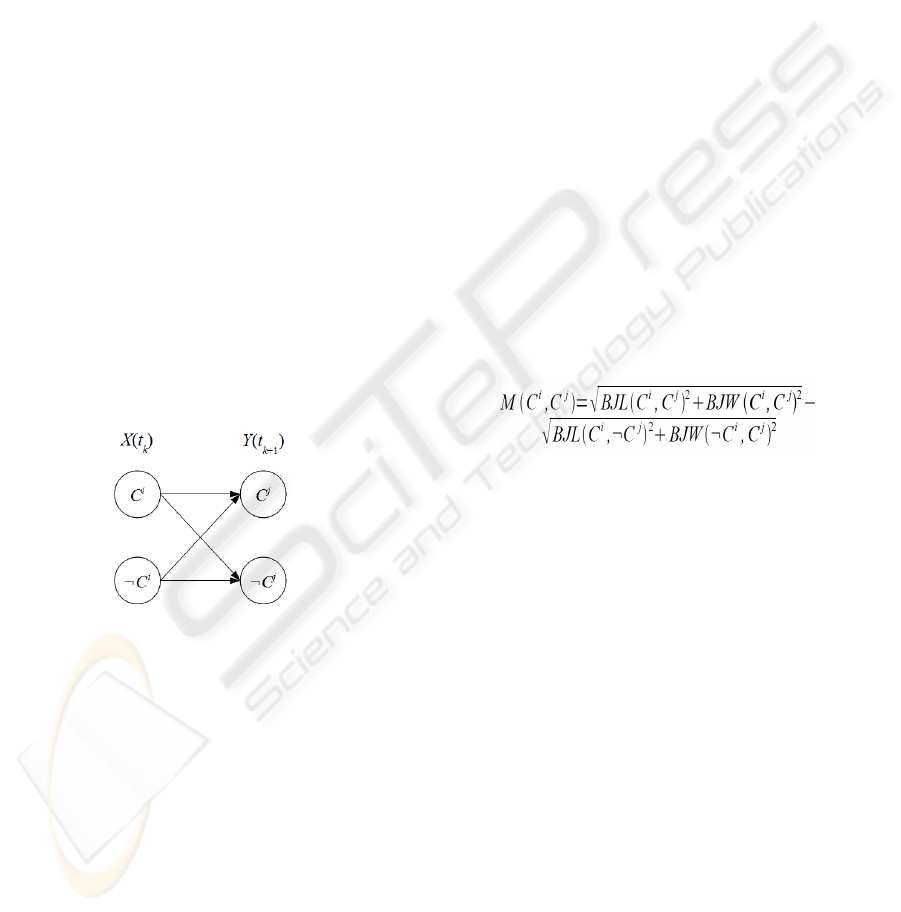
The TOM4L framework proposes also the BJ-
Measure (Benayadi, 2008) that evaluates the
homogeneity of the crisscross of the occurrences of
two observation classes C
i
and C
j
in a sequence. This
measure considers two abstract binary variables X
and Y linked through a discrete binary memoryless
channel of a communication system (Shannon,
1949), where X(t
k
) takes a value C
x
in {C
i
,¬C
i
} and
Y(t
k+1
) a value C
y
in {C
j
,¬C
j
} when reading
(Figure 2, where ¬C
a
denotes any class but C
a
).
With this model, a sequence of m occurrences
C
i
(k) is a sequence of m-1 instances r(C
x
→C
y
) of a
relation r(X→Y)
Figure 2: Discrete Binary Memoryless Channel.
The BJ-measure is build on the Kullback-Leibler
distance D(P(Y|X=Ci)||P(Y)) that evaluates the
relation between the distribution of the conditional
probability of Y knowing that X(tk)=Ci and the prior
probability distribution of Y. One of the properties
of this distance is that D(P(Y|X=Ci)||P(Y))=0 when
P(Y| X=Ci)=P(Y) (i.e. P(Y) and P(X) are
independent). The BJ-measure decomposes the
Kullback-Leibler distance in two terms around the
independence point. The BJL-measure BJL(C
i
→C
j
)
of binary relation r(C
i
→C
j
) is the right part of the
Kullback-Leibler distance D(P(Y|X=C
i
)||P(Y)) so
that:
• P(Y=C
j
|X=C
i
)<P(Y=C
j
) ⇒ BJL(C
i
, C
j
)=0
• P(Y=C
j
|X=C
i
)≥P(Y=C
j
) ⇒
BJL(C
i
→C
j
)= D(P(Y|X=C
i
)||P(Y))
The BJL(C
i
→C
j
) is non-zero when the observation
C
i
(k) provides some information about the
observation C
j
(k). Symmetrically, when
BJL(C
i
→C
j
)<0, the observation C
i
(k) provides some
information about ¬C
j
(k). The BJL-measure
BJL(C
i
→¬C
j
) of a binary relation r(C
i
→¬C
j
) is then
the left part of the Kullback-Leibler distance:
• P(Y=C
j
|X=C
i
)<P(Y=C
j
) ⇒
BJL(C
i
→¬C
j
)=D(P(Y|X=C
i
)||P(Y))
• P(Y=C
j
|X=C
i
)≥P(Y=C
j
) ⇒ BJL(C
i
→¬C
j
)= 0
Consequently:
D(P(Y|X=C
i
)||P(Y))=BJL(C
i
→C
j
)+BJL(C
i
→¬C
j
) (3)
Similarly, the BJW-measure evaluates the
information distribution between the predecessors
(C
i
(k) or ¬C
i
(k)) of an observation C
j
(k+1) at time
t
k+1
:
D(P(X|Y=C
j
)||P(X))=BJW(C
i
→C
j
)+BJW(C
i
→¬C
j
)(4)
Because (P(C
j
|C
i
)<P(C
j
))⇔(P(C
i
|C
j
)<P(C
i
)), the two
measures are null at the same independence point
and can be combined in a single measure called the
BJM-measure which is the norm vector of
BJL(C
i
→C
j
) and BJW(C
i
→C
j
):
(5)
The BJ-Measure is not justifiable when the
θ
i,j
= n
i
/n
j
is greater of 4 or less than ¼ (Benayadi, 2008). This
property is called the
θ
property. In most real world
cases, when this condition is satisfied, the M(C
i
→C
j
)
value is not zero but the eventual relation r(C
i
→C
j
)
can not be justified with the BJ-measure.
The main property of the BJ-measure is the
following: M(C
i
→C
j
) > 0 means that knowing the
timed observation distribution of the C
i
class brings
information about the timed observation distribution
of the C
j
class. Consequently, when the BJ-measure
of a relation r(C
i
→C
j
)≤0, is negative or null, the
relations can not be used to build the structure of a
dynamic Bayesian network.
In other words, considering the positive values
only, the BJ-measure M(C
i
→C
j
) satisfies the three
following properties:
1. Dissymmetry:
M(C
i
→C
j
)≠M(C
j
→C
i
) (generally)
2. Positivity: ∀ C
i
, C
j
, M(C
i
→C
j
) ≥ 0
3. Independence:
M(C
i
→C
j
)=0 ⇔ C
i
and C
j
are independant (i.e.
P(C
j
|C
i
)=P(C
j
))
LEARNING DYNAMIC BAYESIAN NETWORKS WITH THE TOM4L PROCESS
355
4. Triangular inequality:
M(C
i
→C
j
) < M(C
i
→C
k
) + M(C
k
→C
j
)
This latter property can be used to reason with the
BJ-measure to deduce the structure of a dynamic
Bayesian network.
4 LEARNING PRINCIPLES
Let us consider a set R={…, r(C
i
→C
j
), …} of n
binary relations. The operation that remove a binary
relation r(C
i
→C
j
) from the set R is denoted
Remove(r(C
i
→C
j
)): R ← R – { r(C
i
→C
j
) }.
The positivity property leads to remove the
r(C
i
→C
j
) relations having a negative value of the
BJ-measure (“Positivity rule”):
• Rule 1 : ∀r(C
i
→C
j
)∈R, M(C
i
→C
j
)≤0 ⇒
Remove(r(C
i
→C
j
))
The dissymmetry property allows deducing the
orientation of a hypothetical relation between two
timed observation classes C
i
and C
j
:
• Rule 2:
∀r(C
i
→C
j
), r(C
j
→C
i
)∈R,
M(C
i
→C
j
)>BJM(C
j
→C
i
) ⇒ Remove(r(C
j
→C
i
))
This rule means that when M(C
i
→C
j
)>M(C
j
→C
i
),
the C
i
class brings more information about the C
j
class than the reverse. The relation r(C
j
→C
i
) can
then be removed from the set R without any
consequence. This rule is so called the “orientation
rule”.
C
i+1
C
i
BJM(C
i
→C
i+1
)
C
j
BJM(C
i+1
→C
i+2
)
BJM(C
j
→C
i
)
C
i+2
C
i+n
BJM(C
i+n
→C
j
)
…
C
i+1
C
i
BJM(C
i
→C
i+1
)
C
j
BJM(C
i+1
→C
i+2
)
BJM(C
j
→C
i
)
C
i+2
C
i+n
BJM(C
i+n
→C
j
)
…
Figure 3: Loops.
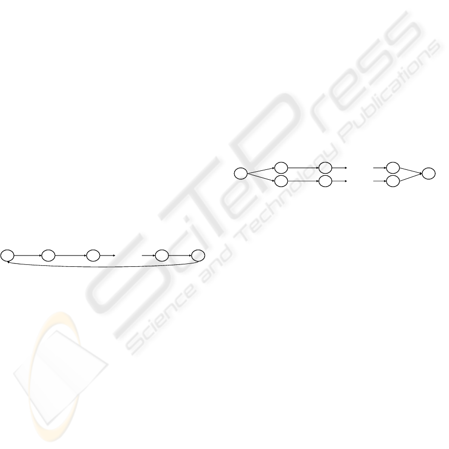
Now, let us consider a set R={r(C
i
→C
i+1
),
r(C
i+1
→C
i+2
), ..., r(C
i+n
→C
j
), r(C
j
→C
i
)} of n+2
binary relations defining a loop (Figure 2) where:
• ∀r(C
x
→C
y
) ∈ R, M(C
x
→C
y
) > 0
The problem of the set R is that computing the
distribution of a class C
x
requires knowing its
distribution: loops must then be avoided. In other
words, a relation r(C
i
→C
j
) must be removed from R
to break the loop. To solve this problem, the idea is
to used the monotonous property of the BJ-measure:
finding two of class C
i
and C
j
so that the BJ-measure
of the relation r(C
i
→C
j
) is the lowest of the loop
(“Loop Rule”):
• Rule 3: ∀r(C
x
→C
y
)∈R, ∃r(C
i
→C
j
)∈R, x≠i, y≠j,
M(C
x
→C
y
)>BJM(C
i
→C
j
) ⇒ Remove(r(C
i
→C
j
))
When M(C
x
→C
y
)=M(C
i
→C
j
)), any of the relations
can be removed. The extreme case of loop can be
find in a set R containing a reflexive relation
r(C
i
→C
i
) where M(C
i
→C
i
)>0. Rule 3 must then be
adapted to this extreme (but frequent) case
(“Reflexivity rule”):
• Rule 4: ∀r(C
i
→C
i
) ∈ R, BJM(C
i
→C
i
) > 0 ⇒
Remove( r(C
i
→C
i
) )
Finally, to build naïve Bayesian Networks, the
algorithm must avoid the multiple paths leading to a
same C
i
class (Figure 3). To avoid this problem, as
for loops, the idea is to use the monotonous property
of the BJ-measure: finding two of class C
i
and C
j
so
that the BJ-measure of the relation r(C
i
→C
j
) is the
lowest of the paths. To use this idea, all the paths
leading to a particular C
i
class must be find in R. Let
us suppose that R contains n paths R
1
⊆R, R
2
⊆R, …,
R
n
⊆R leading to the C
i
class (i.e. each R
i
is of the
form R
i
={r(C
i
→C
k-n
), r(C
k-n
→C
k-n+1
), ..., r(C
k
→C
j
),
r(C
i
→C
l-n
), r(C
l-n
→C
l-n+1
), r(C
l
→C
j
)}. The algorithm
must find the r(C
i
→C
j
) relation with the lowest BJ-
measure to remove it in R (“Transitivity rule”):
• Rule 5: ∀r(C
x
→C
y
)∈R
1
∪R
2
∪…∪R
n
,
∃r(C
i
→C
j
) ∈ R
1
∪R
2
∪…∪R
n
, x≠i, y≠j,
M(C
x
→C
y
)>M(C
i
→C
j
)⇒Remove(r(C
i
→C
j
))
C
k-n
C
i
C
j
C
k-n-1
C
k
…
C
l-m
C
l-m-1
C
l
…
C
k-n
C
i
C
j
C
k-n-1
C
k
…
C
l-m
C
l-m-1
C
l
…
Figure 4: Multiple Paths.
Again, in case of equality (i.e. BJM(C
x
→C
y
) =
BJM(C
i
→C
j
)), any relation can be removed.
These five rules are necessary (but not sufficient)
to design an algorithm that builds naïve Bayesian
Networks from timed data, but its efficiency
depends mainly of the number of relation in the
initial set R. The TOM4L framework provides the
mathematical tools to remove the relations that can
not play a significant role in the building of a naïve
Bayesian Network.
Given the set R={…, r(C
i
→C
j
), …} of n binary
relations that can be build from a sequence
ω
of
timed observation C
i
(k) defining a set C={C
x
} of
N(C) classes C
x
. The size of the Stochastic
Representation matrix of the TOM4L framework is
then N(C)
⋅
N(C)=N(C)
2
. This provides two ways to
eliminate a relation r(C
i
→C
j
) having no interest for
building a naïve Bayesian Network:
• Test 1: P(C
j
|C
i
)⋅P(C
i
, C
j
)≤1/N(C)
3
⇒ Remove(r(C
i
→C
j
))
This first test compares b
ij
≡P(C
j|
C
i
)⋅P(C
i
, C
j
) with
the “absolute” hazard according to the discrete
binary memoryless chanel (Figure 2): because
ω
defines N(C) classes, when supposing that all the
classes are independent and have the same Poisson
ICSOFT 2010 - 5th International Conference on Software and Data Technologies
356

rate of occurrences, the probability of having an
occurrence C
i
(k) of a C
i
class followed by an
occurrence C
j
(k+1) of the C
j
class is simply
P(C
j
|C
i
)=1/N(C) and the probability of reading a
couple (C
i
(k), C
j
(k+1)) in
ω
is P(C
i
, C
j
)= 1 / N(C)
2
.
So each b
ij
value can be compared with the
“absolute” hazard 1 / (N(C) N(C)
2
).
• Test 2: P(C
j
|C
i
)⋅P(C
i
, C
j
)≤(1/(N(C)⋅P(C
i
)⋅P(C
j
))
⇒ Remove(r(C
i
→C
j
))
This second test defines the “relative” hazard when
supposing that C
i
and C
j
classes are independent. In
that case, the probability P((C
j
(k), C
i
(k+1)) in
ω
of
having a couple (C
i
(k), C
j
(k+1)) in
ω
is P(C
i
)⋅P(C
j
)
and having an occurrence C
i
(k) of a C
i
class, the
hazard is to read any occurrence C
j
(k+1) of the C
j
class: P(C
j
|C
i
)=1/N(C). So each b
ij
value can be
compared with the “relative” hazard
1/(N(C)⋅P(C
i
)⋅P(C
j
)).
The
θ
property of the BJ-measure complete these
two tests to eliminate the relation having no meaning
according to the BJ-measure:
• Test 3:
θ
i,j
>4 ∨
θ
i,j
<1/4 ⇒ Remove(r(C
i
→C
j
))
Within the TOM4L framework, these tree tests
are implemented in the F0/1=[f
ij
] matrix:
• (b
ij
>1/N(C)
3
) ∧ (b
ij
>(1/(N(C)⋅P(C
i
)⋅P(C
j
)) ∧ (1/4
≤
θ
i,j
≤ 4) ⇔ f
ij
= 1
So this lead to the rule number 6:
• Rule 6: ∀r(C
i
→C
j
)∈R,
f
ij
= 0 ⇒ Remove( r(C
i
→C
j
) )
These six rules are used by the algorithm inspired
from Cheng’s method to build a naïve Bayesian
Network from timed data.
5 THE BJM4BN ALGORITHM
The proposed algorithm is called “BJM4BN” for
“BJ-Measure for Bayesian Networks”. This
algorithm takes as inputs a sequence ω of m timed
observation C
i
(k) defining a set Cl={C
x
} of N(Cl)
classes C
x
and an output C
j
class that is the class for
which the DBN is computed. It produces a set
G={…, r(C
i
→C
j
), …} of n binary relations that form
the structure of a naïve Bayesian Network (G, ).
The “BJM4BN” algorithm contains 5 stages. The
first stage computes the Stochastic Representation of
to produce the initial M=[m
ij
] matrix containing
the BJ-measure values m
ij
of the N(Cl)
2
binary
relations r(C
i
→C
j
)) defined by (line 1). Next, the
F0/1=[f
ij
] matrix is computed using test 4 (line 3)
so rule 6 is applied (line 4). Finally, the M matrix is
normalized using rules 1 (line 5.1) and 4 (line 5.2).
Stage 2 computes the list L from the normalized
matrix M. Stage 3 builds recursively the initial G
graph from the C
j
class. This stage uses a recursive
function called “Build(G, C
x
)” where C
x
is the class
the graph of which is to build.
Stage 4 finds and removes the loops in G with
Rule 3. This stage finds all the loops R
i
in G of the
form R
i
≡{r(C
i
→C
i+1
), r(C
i+1
→C
i+2
), ..., r(C
i+n
→C
j
),
r(C
j
→C
i
)} and put them in a set R (line 12). Next, a
new list L
1
is build containing all the relation
r(C
x
→C
y
) in R with its associated m
xy
BJ-measure
value (line 13). All loops R
i
in R are then removed
using Rule 3 (line 14). At the end of this stage, G
contains no more loops. Note that the L
1
list being
global (i.e. containing all the relations r(C
x
→C
y
)
participating in a loop), it is guaranty that the set of
removed relation r(C
x
→C
y
) is optimal: it is minimal
and the removed relations are the smallest of the G
graph.
Similarly, stage 5 removes the multiple paths in
the G graph with Rule 5, but the R set contains only
paths R
i
of the form R
i
≡{r(C
i
→C
k-n
), r(C
k-n
→C
k-n+1
),
..., r(C
k
→C
j
), r(C
i
→C
l-n
), r(C
l-n
→C
l-n+1
), ...,
r(C
l
→C
j
)} (line 16). It is guaranty that the set of
removed relation r(C
x
→C
y
) is optimal.
// Stage 1
1. Compute the
M=[m
ij
] matrix
2. ∀i=0…N(Cl), ∀j=0…N(Cl), f
ij
=0
3. ∀i=0…N(Cl), ∀j=0…N(Cl),
(b
ij
>1/N(C)
3
)∧(b
ij
>(1/(N(C)⋅P(C
i
)⋅P(C
j
)
)∧(1/4≤
θ
i,j
≤ 4) ⇒ f
ij
=1
4.
M=M⋅F0/1
5. ∀i=0…N(Cl), ∀j=0…N(Cl),
5.1. m
ij
≤0 ⇒ m
ij
=0 // rule 1
5.2. i=j ⇒ m
ij
=0 // rule 4
// Stage 2
6.
L={
φ
}
7.
∀i=0…N(Cl), ∀j=0…N(Cl), m
ii
>0,⇒
L=L+{(r(C
i
→C
j
), m
ii
)}
// Stage 3
8. C
x
=C
j
, G={
φ
}
9. ∀
r(C
y
→C
x
))∈L ⇒ G=G+{r(C
y
→C
x
)}
10. Build(G, C
x
){
∀
r(C
y
→C
x
))∈G, ∀r(C
z
→C
y
))∈L,
G=G+{
r(C
z
→C
y
)}
Build(G, C
y
)
}// End Build Function
// Stage 4
11. R={
φ
}
12. ∀R
i
⊆G, R
i
≡{r(C
i
→C
i+1
), r(C
i+1
→C
i+2
),
..., r(C
i+n
→C
j
), r(C
j
→C
i
)} ⇒
R=R+{R
i
}
13. ∀R
i
∈R, ∀r(C
x
→C
y
)∈R
i
, r(C
x
→C
y
)∉L
1
⇒
L
1
=L
1
+{(r(C
x
→C
y
), m
xy
)}
LEARNING DYNAMIC BAYESIAN NETWORKS WITH THE TOM4L PROCESS
357

14. While R≠{
φ
} repeat
. ∃r(C
x
→C
y
)∈L
1
, m
xy
= Min(m
ij
, L
1
)
∀R
i
∈R, ∃r(C
x
→C
y
)∈R
i
⇒
R=R-{R
i
}
G=G–{r(C
x
→C
y
)}
L
1
=L
1
-{(r(C
x
→C
y
), m
xy
)}
//Stage 5
15. R={
φ
}
16. ∀R
i
⊆G,
R
i
≡{r(C
i
→C
k-n
), r(C
k-n
→C
k-n+1
), ...,
r(C
k
→C
j
), r(C
i
→C
l-n
), r(C
l-n
→C
l-n+1
),
..., r(C
l
→C
j
)} ⇒ R=R+{R
i
}
17. ∀R
i
∈R,
∀r(C
x
→C
y
)∈R
i
, r(C
x
→C
y
)∉L
1
⇒
L
1
=L
1
+{(r(C
x
→C
y
), m
xy
)}
18. While R≠{
φ
} repeat
∃r(C
x
→C
y
)∈L
1
, m
xy
= Min(m
ij
, L
1
)
∀R
i
∈R, ∃r(C
x
→C
y
)∈R
i
⇒
R=R-{R
i
}
G=G–{r(C
x
→C
y
)}
L
1
=L
1
-{(r(C
x
→C
y
), m
xy
)}
Stage 6 computes the conditional probabilities tables
for G and finalizes the algorithm. The computing of
the Conditional Probabilities Tables ( CP Tables) is
based on the numbering table N=[n
ij
] of the
Stochastic Representation of the sequence. The
following property is a consequence of the model of
the discrete memoryless communication channel
(Figure 2):
• P(Y=C
o
| X=C
i
) + P(Y=¬C
o
| X=C
i
) = 1.
The computing of uses this property (for
simplicity, P(C
y
|C
x
) is rewritten P(y|x)). For a root
node C
x
:
• P(x)=(Σ
j
n
xj
) / Σ
i
Σ
j
n
ij
For a single relation r(C
x
→C
y
):
P(y|x) = n
xy
/ (Σ
j
n
yj
)
P(y|¬x) = ((Σ
i
n
iy
)-n
xy
) / (Σ
i
Σ
j
n
ij
–(Σ
j
n
xj
))
For a set R={r(C
x
→
jy
), r(C
z
→C
y
)} of two relations
converging to the same C
y
class:
• P(y|x,z) = (n
xy
+n
zy
) / (Σ
j
n
xj
+Σ
j
n
zj
)
• P(y|¬x,z) = (Σ
i
n
iy
-n
xy
) / (Σ
i
Σ
j
n
ij
-Σ
j
n
xj
)
• P(y|x,¬z) = (Σ
i
n
iy
-n
zy
) / (Σ
i
Σ
j
n
ij
-Σ
j
n
zj
)
• P(y |¬x,¬z) = (Σ
i
n
iy
-n
xy
-n
zy
) / (Σ
i
Σ
j
n
ij
-Σ
j
n
xj
-Σ
j
n
zj
)
6 A THEORETICAL EXAMPLE
This section illustrates the usage of the proposed
algorithm on the theoretical car example of (Le Goc,
2007). This example is inspired from the (simple)
car technical diagnosis knowledge base of
(Schreiber, 2000) (Figure 5).
Figure 5 shows a knowledge base of 9 rules that can
be used to diagnose a (very simplified) car. These
rules provide the reasons that might affect the car to
stop functioning: a car might “stops” or “does
fuel tank
empty
battery
low
battery dial
zero
gas dial
zero
power
off
engine behavior
does not start
engine behavio
r
stops
gas in engine
false
fuse
blow n
fuse inspection
broken
1
23
45
6
78 9
Figure 5: Car Diagnosis Knowledge Base.
not start” if the fuse is blown or the battery is low or
the fuel tank is empty.
Using the TOM4D methodology, the underlying
structural model of the system considered in this
knowledge base is provided in Figure 6. This figure
shows a set of connected components c
i
and defines
a set of variables x
i
. The evolution of variable x
i
denoted with functions of time x
i
(t).
c7
electric_
alimentation
c8
gas_
alimentation
c9
engine
c6
gas_dial
c5
battery_dial
c4
fuse_inspection
c1
fuse
c2
battery
c3
fuel_tank
x1(t)
x2(t)
x3(t)
x9(t)
x8(t)
x7(t)
x6(t)
x5(t)
x4(t)
c7
electric_
alimentation
c8
gas_
alimentation
c9
engine
c6
gas_dial
c5
battery_dial
c4
fuse_inspection
c1
fuse
c2
battery
c3
fuel_tank
x1(t)
x2(t)
x3(t)
x9(t)
x8(t)
x7(t)
x6(t)
x5(t)
x4(t)
Figure 6: Structural Model of the Car Example.
TOM4D methodology considers that the variables
x
4
, x
5
, and x
6
are associated to the sensor components
c
4
, c
5
and c
6
and these components never failed. So
this figure defines a set X={ x
1
, x
2
, x
3
, x
7
, x
8
, x
9
} of 6
variables. The values of these variables are a set of
constants: Δ={ Δx1={Blown, Not_Blown},
Δx2={Low, Not_Low}, Δx3={Empty, Not_Empty},
Δx7={On, Off}, Δx8={True, False}, Δx9={Start,
Does_Not_Start} }. It is to note that (Le Goc, 2007)
eliminates the constant “Stops”: in the TOM4D
ICSOFT 2010 - 5th International Conference on Software and Data Technologies
358
framework, this corresponds to rewrite the constant
“Stops” as “Does_Not_Start”.
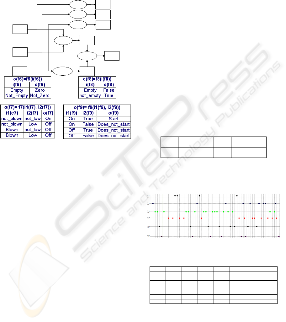
Figure 7 shows the functional model of the car
according to the TOM4D methodology.
f7
f8
f9
f6
f5
f4
x3
x1
x2
x8
x7
x9
x4
x5
x6
f7
f8
f9
f6
f5
f4
x3
x1
x2
x8
x7
x9
x4
x5
x6
Figure 7: Functional Model of the Car Example.
A functional model is an organized set of logical
relations between the possible values the variables
can take over time. The functions are denoted at the
right of Figure 7 and are specified at the left
(function f
4
and f
5
being similar to function f
6
, they
are not specified in the figure).
The role of the Bayesian Network <G, >to
learn is to make a link between the probabilities of
the value of a set X of variables. The discovered
Bayesian network must then be compatible with the
functional model of Figure 7.
Because the “BJM4BN” algorithm works on
timed data, a sequence must be built according to
rules 2, 3, 6, 7 and 8 of the knowledge base of
Figure 5. To this aim, let us suppose that the car is
monitored, the abnormal behaviour of the car can be
defined with a set Ω={
ω
1
,
ω
2
,
ω
3
} of three models of
sequences:
•
ω
1
= {x
1
(t
1
)=Blown, x
7
(t
1
+Δt
7
)=Off,
x
9
(t
1
+Δt
7
+Δt
9
)=Does_Not_Start}
•
ω
2
= {x
2
(t
2
)=Low, x
7
(t
2
+Δt
7
)=Off,
x
9
(t
2
+Δt
7
+Δt
9
)=Does_Not_Start}
•
ω
3
= {x
3
(t
3
)=Empty, x
8
(t
3
+Δt
8
)=False,
x
9
(t
3
+Δt
8
+Δt
9
)=Does_Not_Start}
These sequences define a set Cl={C
i
} of 6
observation classes, each being a singleton: Cl={C
1
= {(x
1
, Blown)}, C
2
= {(x
2
, Low)}, C
3
= {(x
3
,
Empty)} C
7
= {(x
7
, Off)}, C
8
= {(x
8
, false)}, C
9
=
{(x
9
, Does_Not_Start)}}
Consequently, each constant
δ
i
of Δ being linked
with a unique variable x
i
of X, there is a bijection
between a class C
i
and a variable x
i
. The three
sequences of the set Ω can be rewritten in terms of
the class occurrences:
•
ω
1
= {C
1
(t
1
), C
7
(t
1
+Δt
7
), C
9
(t
1
+Δt
7
+Δt
9
)}
•
ω
2
= {C
2
(t
2
), C
7
(t
2
+Δt
7
), C
9
(t
2
+Δt
7
+Δt
9
)}
•
ω
3
= {C
3
(t
3
), C
8
(t
3
+Δt
8
), C
9
(t
3
+Δt
8
+Δt
9
)}
These sequences will be used to produce a
theoretical sequence according to the method
described in [Bouché, 2008]. To this aim, let us
assign hand probabilities to the occurrence of each
observation classes with the following principle: the
observations of the C
1
class (x
1
(t
1
)=Blown) are less
probable to happen than the observations of the C
2
class (x
2
(t
2
)=Low), while the occurrences of the C
3
class (x
3
(t
3
)=Empty) are more frequent (with
carefree driver for example). This lead for example
to the probabilities of Table 1:
Table 1: Prior Probabilities of the car example.
P(
C
1
)P(
C
2
)P(
C
3
)P(
C
7
) P(
C
8
) P(
C
9
)
0.05 0.15 0.3 0.2 0.2 0.1
According to the method of [Bouché, 2008], these
probabilities and the three models of sequence of Ω
allow building a sequence
ω
of 100 occurrences
(Figure 8) that satisfies the probabilities of Table 1.
Figure 8: Theoretical Sequence (beginning).
Table 2: The numbering table N between variables.
N x1x2x3x7x8x9TOTAL
x1 1004005
x2
11291014
x3
168411030
x7
12822520
x8
13803520
x9 02413010
Total
5143020201099
The numbering matrix N computed from the
sequence
ω
is given in Table 2. Next, the M matrix
(Table 3), the B matrix (Table 4, where each cells is
multiplied by 1000 to have readable values) and the
θ matrix (Table 5) are computed to produce the F0/1
matrix (Table 6) that implements the rule 6.
LEARNING DYNAMIC BAYESIAN NETWORKS WITH THE TOM4L PROCESS
359
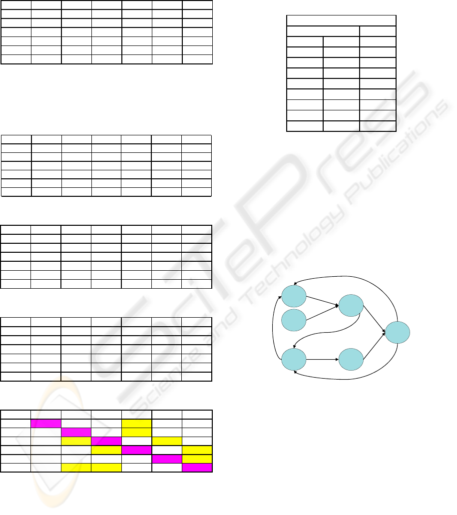
The M⋅F0/1 matrix is then computed and normalized
(Table 7) using rule 1 (pink cells) and rule 4
Table 3: The M Matrix for the Car Example.
M x1x2x3x7x8x9
x1
0.3112 -0.7698 -1.4340 0.3319 -1.0257 -0.5980
x2
0.0217 -0.0629 -0.0851 0.1386 -0.1434 -0.7709
x3
-0.0386 0.0156 -0.0016 -0.0214 0.0343 -1.2864
x7
0.0000 -0.0168 0.0081 -0.0639 -0.0639 0.1087
x8
0.0000 0.0005 0.0081 -0.9955 -0.0112 0.1087
x9
-0.5980 0.0177 0.0124 -0.0749 0.0231 -0.6683
(the yellow cells defines the orientation of a relation
r(x
i
→x
j
)). This achieves the first stage of the
BJT4BN algorithm.
Table 4: The B(*1000) matrix for the car Example.
B*1000 x1 x2 x3 x7 x8 x9
x1
20.20 0.00 0.00 323.23 0.00 0.00
x2
7.22 7.22 28.86 584.42 7.22 0.00
x3
3.37 121.21 215.49 53.87 407.41 0.00
x7
5.05 20.20 323.23 20.20 20.20 126.26
x8
5.05 45.45 323.23 0.00 45.45 126.26
x9
0.00 40.40 161.62 10.10 90.91 0.00
Table 5: The Matrix for the car Example.
T x1x2x3x7x8x9
x1
1 0.35714 0.16667 0.25 0.25 0.5
x2 2.8 1 0.46667 0.7 0.7 1.4
x3 6 2.14286 1 1.5 1.5 3
x7
4 1.42857 0.66667 1 1 2
x8 4 1.42857 0.66667 1 1 2
x9 2 0.71429 0.33333 0.5 0.5 1
Table 6: The F0/1 Matrix for the car Example.
F0/1 x1 x2 x3 x7 x8 x9
x1
100100
x2
000100
x3
010010
x7
001001
x8
001001
x9
011010
Table 7: Normalized M Matrix for the Car Example.
Norm Mx1x2x3x7x8x9
x1
0.0000 0.0000 0.0000 0.3319 0.0000 0.0000
x2
0.0000 0.0000 0.0000 0.1386 0.0000 0.0000
x3 0.0000 0.0156 0.0000 0.0000 0.0343 0.0000
x7 0.0000 0.0000 0.0081 0.0000 0.0000 0.1087
x8 0.0000 0.0000 0.0081 0.0000 0.0000 0.1087
x9
0.0000 0.0177 0.0124 0.0000 0.0231 0.0000
The second stage of the algorithm computes the L
list that contains only the yellow cells of the
normalized M matrix. The Table 8 provides the L list
when sorted with decreasing values of the BJ-
measure m
ij
= M(x
i
→x
j
) of the corresponding
relation r(x
i
→x
j
). The third stage transforms the
normalized M matrix in the initial G graph with a
depth first algorithm (Figure 9).
Stage 4 is dedicated to find and remove the
eventualloops in the initial G graph.
Table 8: The L list of the Car Example.
i
j
mi
j
x1 x7 0.3319
x2 x7 0.1386
x7 x9 0.1087
x8 x9 0.1087
x3 x8 0.0343
x9 x2 0.0177
x3 x2 0.0156
x9 x3 0.0124
x7 x3 0.0081
L = {r(i, j), mij}
The initial G graph of the car example contains a lot
of loops: all the relations participates at least one
loop except the r(x
1
→x
7
) relation. The loops are
suppressed with the iterative removing of the
r(x
i
→x
j
) relations with the minimal BJ-measure m
ij
.
To this aim, the algorithm duplicates the L list
without the r(x
1
→x
7
) relation to constitute the L
1
list.
It is then easy to see that the firstly removed relation
is r(x
7
→x
3
), and that the algorithm will successively
remove the r(x
9
→x
3
) and the r(x
3
→x
2
) relations
(Figure 10).
x
9
x
7
x
8
x
1
x
3
x
2
Figure 9: Initial G Graph for the Car Example.
The resultant G graph having no multiple paths, the
stage 5 modifies nothing. The final stage of the
algorithm is dedicated to the computing of the CP
Tables from the N matrix (Table 2) with the
equations provided in section 5. For the two root
nodes x
1
, x
2
and x
3
:
• P(x
1
) = 5 / 99 ≈ 0.050
• P(x
2
) = 14 / 99 ≈ 0.141
• P(x
3
) = 30 / 99 ≈ 0.303
For the single relation r(x
3
→x
8
):
• P(x
8
|x
3
) = 11 / 30 ≈ 0.366
• P(x
8
|¬x
3
) = (20-11) / (99-30) ≈ 0.130
For the converging node x
7
corresponding to the set
R
7
={r(x
1
→x
7
), r(x
2
→x
7
}:
ICSOFT 2010 - 5th International Conference on Software and Data Technologies
360
• P(x
7
|x
1
,x
2
) = (4+9) / (5+14) ≈ 0.684
• P(x
7
|¬x
1
,x
2
) = (20-4) / (99-5) ≈ 0.170
• P(x
7
|x
1
,¬x
2
) = (20-9) / (99-14) ≈ 0.129
• P(x
7
|¬x
1
,¬x
2
) = (20-4-9) / (99-5-14) ≈ 0.087
For the converging node x
9
corresponding to the set
R
9
={r(x
7
→x
9
), r(x
8
→x
9
}:
• P(x
9
|x
7
,x
8
) = (5+5) / (20+20) ≈ 0.250
• P(x
9
|¬x
7
,x
8
) = (10-5) / (99-20) ≈ 0.063
• P(x
7
|x
1
,¬x
2
) = (10-5) / (99-20) ≈ 0.063
• P(x
7
|¬x
1
,¬x
2
) = (10-5-5) / (99-20-20) =0
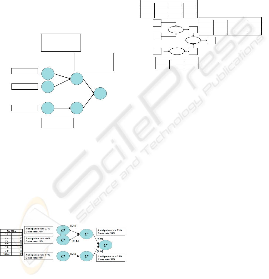
This leads to the final naïve Bayesian Network for
the car example (Figure 10), which is compatible
with the functional model of Figure 7.
P(x2) = 0,14
P(x1) = 0,05
P(x3) = 0,30
P(x7 | x1, x2) = 0.684
P(x7 | x1, ¬x2) = 0.129
P(x7 | ¬ x1, x2) = 0.170
P(x7 | ¬x1, ¬x2) = 0.087
P(x9 | x7, x8) = 0.250
P(x9 | x7, ¬x8) = 0.063
P(x9 | ¬ x7, x8) = 0.063
P(x9 | ¬x7, ¬x8) = 0.000
P(x8 | x3) = 0.367
P(x8 | ¬x3) = 0.130
x
9
x
7
x
8
x
1
x
3
x
2
P(x2) = 0,14
P(x1) = 0,05
P(x3) = 0,30
P(x7 | x1, x2) = 0.684
P(x7 | x1, ¬x2) = 0.129
P(x7 | ¬ x1, x2) = 0.170
P(x7 | ¬x1, ¬x2) = 0.087
P(x9 | x7, x8) = 0.250
P(x9 | x7, ¬x8) = 0.063
P(x9 | ¬ x7, x8) = 0.063
P(x9 | ¬x7, ¬x8) = 0.000
P(x8 | x3) = 0.367
P(x8 | ¬x3) = 0.130
x
9
x
7
x
8
x
1
x
3
x
2
x
9
x
7
x
8
x
1
x
3
x
2
Figure 10: Bayesian Network for the Car Example.
Naturally, this result comes from the way the
sequence has been made: the Figure 11 shows the
signature tree of the C
9
class as provided by the
“BJT4S” algorithm of the TOM4L tools. This tree
allows recognizing the 10 observations of the C9
class in the sequence (i.e. the cover rate is equal to
100%): 5 observations of the C
9
class are recognized
by the {r(C
2
, C
7
, [0, 6s]), r(C
1
, C
7
, [0, 4s]), r(C
7
, C
9
,
[0, 6s])} signature, the other 5 observations being
recognized by the {r(C
3
, C
8
, [0, 6s]), r(C
8
, C
9
, [0,
12s])} signature.
Figure 11: Signature tree of the C
9
class.
Despite of the simplicity of the knowledge base of
the car example (Figure 5), this shows a posteriori
the difficulty to compute the car example Bayesian
network from the observations of the sequence.
The Bayesian Network of Figure 11 allows the
building of the functional model for the car example
of Figure 12: this functional model is identical to the
functional model Figure 7, but it adds probabilities
to the functions f
7
, f
8
and f
9
. These probabilities
provide some confidence about the existence of the
corresponding functions. This example show the
way the TOM4D methodology and the TOM4L
process complete together.
x
9
x
7
x
8
x
1
x
3
x
2
f
7
f
8
f
9
x
3
x
8 P (
x
8)
Empty False 37%
Not_Empty True 87%
x 8=f 8(x 3)
x1 x2 x7
P (
x
7)
Not_Blown Not_Low On 91%
Not_Blown Low Off 17%
Blown Not_Low Off 13%
Blown Low Off 68%
x 7=f 7(x 1, x 2)
x7 x8 x9
P (
x
9)
On True Start 100%
On False Does_Not_Start 6%
Off True Does_Not_Start 6%
Off False Does_Not_Start 25%
x 9=f 7(x 7, x 8)
x
9
x
7
x
8
x
1
x
3
x
2
f
7
f
8
f
9
x
9
x
7
x
8
x
1
x
3
x
2
f
7
f
8
f
9
x
3
x
8 P (
x
8)
Empty False 37%
Not_Empty True 87%
x 8=f 8(x 3)
x1 x2 x7
P (
x
7)
Not_Blown Not_Low On 91%
Not_Blown Low Off 17%
Blown Not_Low Off 13%
Blown Low Off 68%
x 7=f 7(x 1, x 2)
x7 x8 x9
P (
x
9)
On True Start 100%
On False Does_Not_Start 6%
Off True Does_Not_Start 6%
Off False Does_Not_Start 25%
x 9=f 7(x 7, x 8)
Figure 12: Functional Model for the Car Example.
This example shows the simplicity and the
efficiency of the BJM4BN algorithm. The
complexity of the algorithm is proportional with the
number of timed data in the given set of sequences
and the number of class N(C) in . This is to be
compared with the exponential complexity of the
methods of the dependency analysis category.
The next section shows the use of the
“Transitivity rule” and the ease of use of the
proposed algorithm in an industrial environment.
7 REAL WORLD APPLICATION
The Apache system is a clone of Sachem, the
knowledge based systems that The Arcelor Group,
one of the most important steal companies in the
world, has developed to monitor and diagnose its
production tools (Le Goc, 2004). Apache aims at
controlling a zinc bath, a hot bath containing a liquid
mixture of aluminum and zinc continuously fed with
aluminum and zinc ingots in which a hot steel strip
is immerged. Apache monitors and diagnoses around
11 variables and is able to detect around 24 types of
alarms. The analyzed sequence ω contains 687
events of 13 classes for 11 discrete variables. The
counting matrix N contains then 156 cells n
ij
(Bouché, 2005), (Le Goc, 2005).
The node of interest being 1006, the initial G graph
resulting from stage 3 of the “BJM4BN” algorithm
is given in Figure 13. This graph having no loops,
LEARNING DYNAMIC BAYESIAN NETWORKS WITH THE TOM4L PROCESS
361
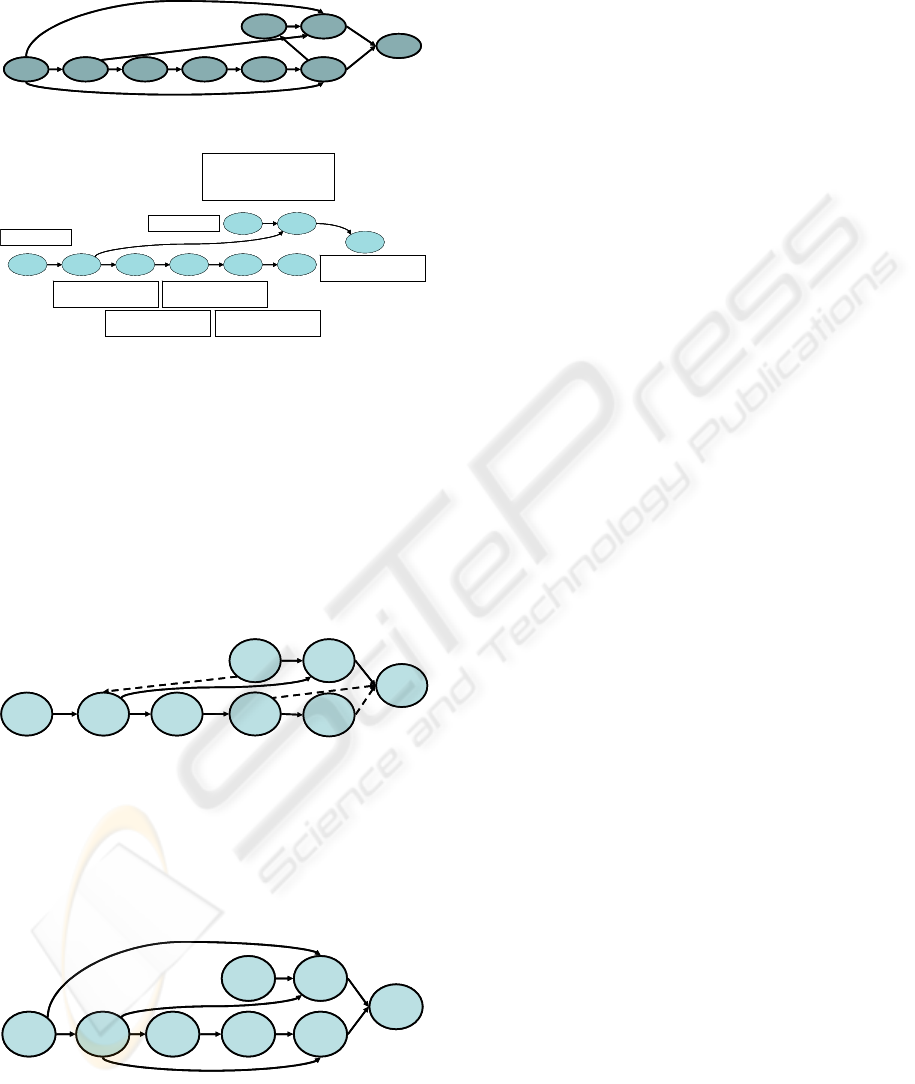
the stage 4 modify noting and stage 5 builds the final
G graph of Figure 14.
1006
1001
1020
1031
10261004 10141002 1024
1006
1001
1020
1031
10261004 10141002 1024
Figure 13: Initial G graph.
P(1031) = 0,176
P(1004) = 0,026
P(1014 | 1002) = 0.385
P(1014 | ¬1002) = 0.024
P(1026 | 1014) = 0.400
P(1026 | ¬1014) = 0.010
P(1024 | 1026) = 0.059
P(1024 | ¬1026) = 0.025
P(1001 | 1031, 1002) = 0.088
P(1020 | 1031, ¬1002) = 0.053
P(1020 | ¬ 1031, 1002) = 0.053
P(1020 | ¬1031, ¬1002) = 0.048
P(1020 | 1024) = 0.120
P(1020 | ¬1024) = 0.033
P(1006 | 1001) = 0.385
P(1006 | ¬1001) = 0.037
1006
1001
1020
1031
10261004 10141002 1024
1006
1001
1020
1031
10261004 10141002 1024
Figure 14: Final G graph.
Figure 15 shows a handmade sketch of the
functional model of the galvanization bath problem
produced by the experts of the Arcelor Group in
2003. The dotted lines in the graph indicate the
expert’s relations that are not included in the final G
graph of Figure 14: the G graph is all contained in
the expert’s graph. But the expert’s graph does not
contain the 1024 class: corresponding to an operator
query for a chemical analysis, this class has been
removed by experts.
1020
1014
1026
1006
1002
1031 1001
1004
1020
1014
1026
1006
1002
1031 1001
1004
Figure 15: Handmade graph of experts.
Finally, the Figure 16 shows the graph made with
the signatures of the 1006 class that can be found in
(Bouché, 2005) and (Le Goc, 2005). The signatures
are produced with specific Timed Data Mining
techniques. This graph is identical to the initial G
graph of Figure 13.
10201014 1026
1006
1002
1031 1001
.1004 10201014 1026
1006
1002
1031 1001
.1004
Figure 17: Handmade graph from 1006 signatures.
The main problem is the disappearance of the
r(1020, 1006) relation in the final G graph. The first
analysis seem to lead to the conclusion that the 1024
class is responsible of the r(1020, 1006) removing.
8 CONCLUSIONS
This paper proposes a new algorithm called the
“BJT4BN” algorithm to learn a Bayesian Network
from timed data.
The originality of the algorithm comes from the
fact that it is designed in the framework of the
Timed Observation Theory. This theory represents a
set of sequences of timed data in a structure, the
Stochastic Representation that allows the definition
of a new information measure called the BJ-
Measure. This paper defines the principles of a
learning algorithm that are based on the BJ-Measure.
The BJT4BN algorithm is efficient both in terms
of pertinence and simplicity. These properties come
from the BJ-measure that provides an operational
way to orient the edges of a Bayesian Network
without the exponential CI Tests of the methods of
the dependency analysis category.
Our current works are concerned with the
combination of the Timed Data Mining techniques
of the TOM4L framework with the “BJT4BN”
algorithm to define a global validation of the
TOM4L learning process.
REFERENCES
Benayadi, N., Le Goc, M., (2008). Discovering Temporal
Knowledge from a Crisscross of Timed Observations.
To appear in the proceedings of the 18th European
Conference on Artificial Intelligence (ECAI'08),
University of Patras, Patras, Greece.
Bouché, P., Le Goc, M., Giambiasi, N., (2005). Modeling
discrete event sequences for discovering diagnosis
signatures. Proceedings of the Summer Computer
Simulation Conference (SCSC05) Philadelphia, USA.
Cheeseman, P., Stutz, J., (1995). Bayesian classification
(Auto-Class): Theory and results. Advances in
Knowledge Discovery and Data Mining, AAAI Press,
Menlo Park, CA, p. 153-180.
Cheng, J., Bell, D., Liu, W., (1997). Learning Bayesian
Networks from Data An Efficient Approach Based on
Information Theory.
Cheng, J., Greiner, R., Kelly, J., Bell, D., Liu, W., (2002).
Learning Bayesian Networks from Data: An
Information-Theory Based Approach. Artificial
Intelligence, 137, 43-90.
Chickering, D. M., Geiger, D., Heckerman, D., (1994).
Learning Bayesian Networks is NP-Hard. Technical
Report MSR-TR-94-17, Microsoft Research, Microsoft
Corporation.
ICSOFT 2010 - 5th International Conference on Software and Data Technologies
362

Cooper, G. F., Herskovits, E., (1992). A Bayesian Method
for the induction of probabilistic networks from data.
Machine Learning, 9, 309-347.
Friedman, N., (1998). The Bayesian structural EM
algorithm. Proceedings of the 14th Conference on
Uncertainty in Artificial Intelligence. Morgan
Kaufmann, San Francisco, CA, p. 129-138.
Heckerman, D., Geiger, D., Chickering, D. M., (1997).
Learning Bayesian Networks: the combination of
knowledge and statistical data. Machine Learning
Journal, 20(3).
Le Goc, M., Bouché, P., and Giambiasi, N., (2005).
Stochastic modeling of continuous time discrete event
sequence for diagnosis. Proceedings of the 16th
International Workshop on Principles of Diagnosis
(DX’05) Pacific Grove, California, USA.
Le Goc, M., (2006). Notion d’observation pour le
diagnostic des processus dynamiques: Application a
Sachem et a la découverte de connaissances
temporelles. Hdr, Faculté des Sciences et Techniques
de Saint Jérôme.
Le Goc, M., Masse, E., (2007). Towards A Multimodeling
Approach of Dynamic Systems For Diagnosis.
Proceedings of the 2
nd
International Conference on
Software and Data Technologies (ICSoft'07),
Barcelona, Spain.
Le Goc, M., Masse, E., (2008). Modeling Processes from
Timed Observations. Proceedings of the 3rd
International Conference on Software and Data
Technologies (ICSoft 2008), Porto, Portugal.
Myers, J., Laskey, K., Levitt, T., (1999). Learning
Bayesian Networks from Incomplete Data with
Stochastic Search Algorithms.
Pearl, J., (1988). Probabilistic Reasoning in Intelligent
Systems: Networks of Plausible Inference. San Mateo,
Calif.: Morgan Kaufmann.
Shannon, C., Weaver, W., (1949). The mathematical
theory of communication. University of Illinois Press,
27:379–423.
LEARNING DYNAMIC BAYESIAN NETWORKS WITH THE TOM4L PROCESS
363
