
THE TASK GRAPH ASSIGNMENT FOR KASKADA PLATFORM
1
Henryk Krawczyk
Electronics, Telecommunications and Informatics Faculty, Gdansk University of Technology
Narutowicza 11/12, Gdansk, Poland
Jerzy Proficz
Academic Computer Center – TASK, Gdansk University of Technology
Narutowicza 11/12, Gdansk, Poland
Keywords: Task assignment, Computation cluster, Multimedia processing.
Abstract: The paper describes a computational model of the KASKADA platform. It consists of two main elements: a
computational cluster, and a task graph. The cluster is represented by a finite set of the nodes with the
specific maximum loads. The graph contains nodes representing tasks to be executed, and the edges
representing continuous data flow between the tasks. The tasks are executed concurrently and the data flows
between them are directed and acyclic. For such a model, the problem of task-to-nodes assignment is
analysed, and two optimisation goals are defined: low cluster fragmentation, and minimum processing
latency. For both problems the heuristic algorithms are described. The simulation results of the described
algorithms are provided, and their evaluation is performed. Finally, the future algorithm improvements are
suggested.
1 INTRODUCTION
Context Analysis of the Camera Data Streams for
Alert Defining Applications platform (Polish
abbreviation: KASKADA, i.e. waterfall) is a
platform supporting services used for multimedia
stream processing. The simple services are directly
related to the computational tasks implementing
concrete processing algorithms, e.g. face
recognition. A complex service is defined as a graph
of simple services, which is transformed to a task
graph (Krawczyk, 2010).
The typical problem of task scheduling is defined
as assignment of a set of task into the set of
computational nodes in a particular order. The tasks
are grouped in the graph as the nodes, where a
directed edge between two tasks t
1
and t
2
indicates
the task t
1
to be finished before the task t
2
is started.
It is proved, the above problem is NP-hard for the
general case, and there exists a polynomial solution
for task scheduling on two computational nodes (El-
Rewini, 1994).
The proposed architecture assumes tasks are
executed continuously, consuming and producing
data streams. Each of them requires concrete
computational power to support provided
functionality. We believe that due to the character of
multimedia stream processing, the tasks require
concurrent execution, and they cannot be queued
and started in the sequence one by one.
We introduce a specific definition of the task-to-
nodes assignment regarding the above constraints.
The task graph is to be assigned to the computational
nodes, which can be free or already partially used,
by already working tasks. In case the task graph
cannot be completely assigned, the platform will
refuse the whole graph. And in case there is more
than one possible complete assignment, the platform
should optimise its selection using one of the
following criteria: minimizing the fragmentation, or
processing latency.
The assignment described above is quite similar
to the well known bin packing problem (BPP)
(Garey, 1979), especially the version with the
variable bin sizes (VBPP) (Haouari, 2009). Typical
BPP minimizes a number of baskets (computational
nodes in our case) used for packing a set of objects
1
The work was realized as a part of MAYDAY EURO
2012 project, Operational Program Innovative Economy
2007-2013, Priority 2, Infrastructure area R&D”.
192
Krawczyk H. and Proficz J. (2010).
THE TASK GRAPH ASSIGNMENT FOR KASKADA PLATFORM.
In Proceedings of the 5th International Conference on Software and Data Technologies, pages 192-197
DOI: 10.5220/0002929401920197
Copyright
c
SciTePress

(tasks). The version with the basket variable sizes
introduces additionally a finite set of basket types
with different sizes. An exact algorithm for (V)BPP
is NP-hard (Garey, 1979).
We would like to emphasize the difference
between the VBPP, and our problem: for VBPP we
can use as many baskets of possible type (size) as
we need, however for the considered assignment,
found in the real environment, the number of each
type is finite. Moreover, the optimisation goals are
different, VBPP minimizes the number of used
baskets and we consider fragmentation (the number
of partially used nodes) or latency in the processing.
In the next section we provide the formal
description of the processing model and assignment
problem. In the third section we consider the
existence of a solution for the problem. The fourth
and fifth sections contain the description of the
proposed heuristic algorithms followed by the
section with their evaluation and finally some
conclusions are provided.
2 THE ASSIGNMENT MODEL
A task graph is defined as a pair G=(T, D), where
T={t
1
, t
2
, … t
N
} is a set of tasks executed during the
processing, and D={d
1
, d
2
, … d
M
} is a set of the
directed edges representing data flow between the
tasks. E.g. edge d
1
=(t
1
, t
2
) indicates the task t
2
receives the data from a stream generated by the task
t
1
. Function Φ: T → N (where N is a set of natural
numbers) denotes the task load: computational
power required for the task to be executed, see
figure 1. We assume the task graph is acyclic and
directed (DAG), where the edge directions indicate
data stream flows.
Φ(t
1
) = 1
Φ(t
2
) = 1
Φ(t
3
) = 2
Φ(t
4
) = 0
Figure 1: Example of tasks-to-nodes assignment.
A computational cluster is represented as a set of
nodes C={c
1
, c
2
, … c
H
}, with the same initial
computational power: ɣ. Each node can have
different available computational power denoted by
a function Г: C → N. E.g. for a cluster with three
nodes the computational power can be as follows:
Г(c
1
)=1, Г(c
2
)=2, Г(c
3
)=2 and ɣ=3. We assume the
inter-node connections are realized by a complete
graph of network links – communication between
any two nodes always requires the same resources
and takes the same time.
M(t
1
) = c
2
M(t
2
) = c
2
M(t
3
) = c
3
M(t
4
) = c
2
Figure 2: Example of tasks-to-nodes assignment.
A tasks-to-nodes assignment is defined as a
function M: T → C, assigning a node c to the task t,
fulfilling the following:
cΓτ
c=τMτ
:
(1),
so the sum of computational load of all nodes
assigned to a node is lower or equal to the actual
computational power. The example of a task graph
(from figure 1) assignment to a cluster with three
nodes is provided in figure 2.
For the assignment algorithms analysis we use
the following assumptions:
Z1. A task graph is a tree.
Z2. A task graph is a tree and only the tasks being
leaves perform computations:
0)(
0)(:
*
T
where ϱ
*
(τ) is a degree of τ node for incoming
edges.
Z3. The computation load of all tasks is 0 or 1:
}1,0{)(
T
(2).
3 THE ASSIGNMENT
EXISTENCE
The first problem considered for the above
assignment definition, is an examination of if it is
possible to make any assignment of a given task
graph to a cluster, formally, it is equal to the
following question: Does there exist any function
complying with the condition (1), for a given task
graph G=(T, D) and a node set C? For instance, the
graph in figure 1 cannot be assigned and executed
using the following cluster: C={c
1
, c
2
, c
3
, c
4
}, where
Г(c
i
)=1 for i=1…4.
The above problem is NP-hard.
t
2
t
1
t
3
t
4
d
1
d
2
d
3
t
2
t
1
t
3
d
1
d
2
d
3
t
4
c
3
c
2
THE TASK GRAPH ASSIGNMENT FOR KASKADA PLATFORM
193

Proof: Even if we assume all cluster nodes have the
same actual computational power equal to initial
power:
)(c
Cc
where
Nk (3),
it is an equivalent to NP-hard optimisation bin
packing problem (BPP). We treat the computational
nodes as the bins, and the tasks as the packed
objects. Let's assume we have the algorithm
checking if h nodes can be used to pack T (objects),
then iterating one-by-one natural numbers
(maximally |T| times, or even log
2
|T| if we use
binary search instead) we would resolve BPP: the
result is the minimal number for which the algorithm
returned a positive answer.
With the assumption Z3, any task can be
assigned for any node c, if Г(c)>0. In such a
simplified case, it is enough to compare the actual
computational power of the cluster (sum of all nodes
actual power) with the sum of task load, to check the
existence of a solution:
CcTt
ct )()( (4).
4 OPTIMIZATION OF CLUSTER
FRAGMENTATION
The fragmentation indicates the number of nodes
partially engaged in task processing. Figure 3 shows
a scenario where a new complex task cannot be
assigned to any node.s
t
?
c2
c3
c1
c4
Г(c
1
)=5
Г(c
1
)=2
Г(c
1
)=4
Г(c
1
)=5
Φ(t) = 6
Figure 3: Example of the cluster fragmentation preventing
from a new task assignment.
To avoid the above problem, we propose the
optimisation goal, where the number of the partially
assigned computation nodes (Г(c)<ɣ) is minimized.
Below we provide the formal definition of the
optimisation according the assumed model.
Let's define M
as a set of all possible
assignments M: T → C fulfilling condition (1).
Optimal solution for optimisation of cluster
fragmentation is a function MM for which the
number of partially used nodes is minimal:
0: >tcΓγcmin
cMt
.M
(5).
The existence of function M is NP-hard problem, so
its optimisation has the same property.
Algorithm 1: Algorithm based on SSP.
We emphasize the difference between the above
optimisation and the one defined for bin packing
problem: minimizing of the used node number. The
following example illustrates this: let's assume the
following task graph: T={t
1
, t
2
, t
3
}, where Φ(t
1
)=2,
Φ(t
2
)=3, Φ(t
3
)=5 and the cluster nodes' set: C={c
1
,
c
2
, c
3
, c
4
}, where Г(c
1
)=5, Г(c
2
)=5, Г(c
3
)=6,
Г(c
4
)=10 and ɣ=10. The optimal solution for VBPP
is as follow: {t
1
, t
2
, t
3
} → c
4
, however the
fragmentation optimisation is: {t
1
, t
2
} → c
1
and {t
3
}
→ c
2
.
Algorithm 2: Algorithm FF/FFD.
In algorithm 1, we define the heuristic using a
subset sum function, based on (Haouari, 2009).
SSP
is a function solving subset sum problem. This
problem is also NP-complete class, so in this case,
the approximation solution can be used (Capara,
2004).
The next proposed group of heuristic algorithms
is based on an intuitive approach, whose common
property is a loop iterating the task set to fit them
1. create a list T* of elements from a set
T
2. for FFD: sort descending T* by function
Φ(.)
3. create a list C*: sorted ascending set
C, by function Г(.)
4. for i = 0 to N
5. for j = 0 to H
6. if Φ(T*
i
) ≤ Г(C*
j
)
7.
make an assignment:
M(T*
i
) := C*
i
8. continue with the next task
9. success condition: for each task
condition in line 6 was true at least
once
1. T
R
:= T
2. create C*: sorted ascending set C,
using Г(.) function
3. for i = 0 to H
4.
c := C*
i
5. T':= SSP(T
R
, Г(c))
6. make an assignment:
T'τ
M(T*
i
):= C*
i
7. T
R
= T
R
\T'
8. success condition: T
R
= Ø
ICSOFT 2010 - 5th International Conference on Software and Data Technologies
194

one by one to the computation nodes. First fit (FF)
algorithm assigns subsequent tasks to the first node
having enough computational power for its
execution, in the first fit descending (FFD) version
of this algorithm it iterates the tasks in descending
order, sorted by Φ(.).
Algorithm 3: Algorithm BF/BFD.
The best fit (BF) algorithm, like FF, iterates the
task set, however the nodes are not assigned one by
one, but they are selected to make best fit:
minimizing the actual power left in the assigned
node. As well as for FFD there is also a version with
the sorted task set. Algorithm 3 presents the detailed
pseudo-code for BF/BFD.
5 OPTIMIZATION
OF PROCESSING LATENCY
Processing latency depends on cooperation among
tasks which are executed. If a cooperated tasks are
assigned to the same node the latency is low because
instead of data marshalling, transfer and
unmarshalling is used only copy operation, see
figure 4.
For further consideration, we take the following
simplifying assumptions:
Z4. All task graph nodes introduce the same
processing latency: L
T
.
Z5. The latency for the edge between two tasks
executed on the same computational node is always
the same and equals: L
N
.
Z6. The latency for the edge between two tasks
executed on different nodes is always the same and
equals: L
E
.
Z7. The latency for the edge between two tasks
inside one node is always lower than between tasks
executed on different nodes: L
E
>L
N
.
c
1
c1 c2
1. copy
1. marshal
2. transfer
3. unmarshal
(a)
(b)
Figure 4: Example of the mappings with (a) low and (b)
high latency due to task assignment to the different
computation nodes.
Let's consider the task graph described in figure
1, it contains three edges and any one of them can be
placed between computational nodes. Figure 5
presents example assignments: M
1
(.) and M
2
(.) - all
edges are separated by the nodes, M
4
(.) - all edges
are in the same node, and M
3
(.) where one edge is
placed between the nodes.
According to the above assumptions, latency of
the event generated in task t
3
after its propagation to
task t
4
is as follows:
for M
1
: L(M
1
, t
3
, t
4
) = L
E
+L
T
+L
E
+L
T
= 2L
E
+2L
T
for M
3
: L(M
3
, t
3
, t
4
) = L
E
+L
T
+L
N
+L
T
= L
E
+L
N
+2L
T
for M
4
: L(M
4
, t
3
, t
4
) = L
N
+L
T
+L
N
+L
T
= 2L
N
+2L
T
According to the assumption Z7:
L(M
1
, t
3
, t
4
) > L(M
3
, t
3
, t
4
) > L(M
4
, t
3
, t
4
).
Below we define L(M, t
1
, t
2
) for task graph G:
E
r
N
r
T
r
LDSD+LDS+LTmax
2
t
1,
tG,R
r
D,
r
T
(6)
where:
t'M=tMDt't,=DS :
,
R(G, t
i
, t
j
) – is a set of subgraphs of graph G,
being the routes between the tasks: t
i
and t
j
.
The above latency function is defined for two
tasks between which its value is computed, we can
also provide such a function L for the whole graph G
and concrete assignment (mapping) M, it is a
maximum latency for any pair of the tasks:
ji
ji
t
t,tM,L
Tt,
max=GM,L
(7).
Assignment optimisation for the processing
latency means selection of such mapping MM,
where the data propagation is minimal:
M,GLmin
.M
(8).
Finding optimal assignment M(.) is NP-hard,
because even checking for its existence has such
property. Because of this, we propose a heuristic
1. create a list T* of elements from a set
T
2. for BFD: sort descending T* by function
Φ(.)
3. for i = 0 to N
4. find cC where Φ(T*
i
) Г(c) and
Г(c) - Φ(T*
i
) is minimal
5. make an assignment: M(T*
i
) := c
6. success condition: for each task
condition in line 4 was true at least
once
THE TASK GRAPH ASSIGNMENT FOR KASKADA PLATFORM
195

t
2
t
1
t
3
t
4
d
1
d
2
d
3
t
2
t
1
t
3
t
4
d
1
d
2
d
3
t
2
t
1
t
3
t
4
d
1
d
2
d
3
c
2
c
3
c
1
c
1
c
2
c
1
M
2
(.) M
4
(.)M
3
(.)
t
2
t
1
t
3
t
4
d
1
d
2
d
3
c
2
c
3
c
1
M
1
(.)
c
4
Figure 5: Task-to-node assignment example.
approach. Algorithm 4: HLT uses a set of tasks
sorted by the topological order and the function
directNeighbours() finding a set of
neighbouring tasks – receiving data from the task
provided as a function argument.
In the algorithm the tasks are assigned to the
computational nodes using the recursion function
matchDepthFirst(), traversing the graph using a
depth-first approach.
Algorithm 4: Heuristic algorithm optimising processing
latency: HLT.
6 EVALUATION
OF THE PROPOSED
ALGORITHMS
For the proposed algorithms we performed the
simulation in conditions close to the real execution
in the target environment – KASKADA platform.
After its analysis we made the following
assumptions:
1. the initial computational power of a node:
ɣ=80 (integer values),
2. the task loads: Φ(t
i
)=1-80 (integer values,
uniform distribution),
3. the number of not assigned nodes (Г()=80): 20,
4. the available computational power of the
partially assigned nodes: Г()=1..79 (uniform
distribution),
5. the number of partially assigned nodes: 8,
6. used SSP algorithm – exact (for the above
condition we could use a dynamic
programming solution)
7. latencies: L
E
=16, L
N
=1, L
T
=32,
8. each task (except the termination ones) has 0-2
outgoing edges (communication with other
tasks).
The above assumptions are related to the
conditions for the assignment module in KASKADA
platform used in project MAYDAY EURO 2012.
However they are general enough to be used for
other applications with possible slight modifications.
Table 1 and figure 6 present the simulation
results for heuristics according to the above
assumptions. They are grouped by the task set sizes:
|T| and show the percent factor α
A
, defined as
follow:
number of experiments when A gave
A
the best solution for the fragmentation
number of experiments for A
1. create list T*: the set T sorted
descending in topological order
2. create list C*: the set C sorted
descending by Г(.) function
3. while T* ≠ do
4.
c := C*
0
5. fv := head(T*)
6. if Φ(fv) > Г(c) then
7. break
8. V := {fv}
9. matchDepthFirst(V, fv, Г(c))
10. foreach cv in V
11. M(cv) := c
12. sort descending list C* by Г(.)
function
13. success condition: T* =
14. procedure matchDepthFirst(V, v,
max)
15. w := 0
16. foreach rv in V
17. w := w+Φ(rv)
18. foreach nv in
directNeighbours(v)
19. if nvT* Φ(nv)+w≤max then
20. V := V{nv}
21. T* := T*\{nv}
22. match(V, nv, max)
ICSOFT 2010 - 5th International Conference on Software and Data Technologies
196
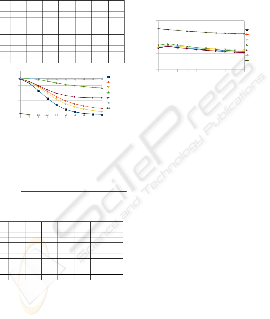
Table 1: Simulation results of the heuristic algorithms for
the factor α.
2468101214161820
0.00%
20.00%
40.00%
60.00%
80.00%
100.00%
120.00%
FF
FFD
BF
BF D
SSP
BF D SS
LAT
Figure 6: Simulation results of the heuristic algorithms for
the factor α. Axis X: task number, axis Y: factor α.
Similarly table 2 and figure 7 present the simulation
results for the algorithms, which are grouped by the
task set sizes: |T|, but showing the percent latency
factor βA, defined as follow:
number of experiments when A gave
A
the best solution for the latency
number of experiments for A
Table 2: Simulation results of the heuristic algorithms for
the factor β.
The number of executed experiments for each
algorithm is 100,000, for each experiment there were
randomly generated task graphs G and cluster states
C: computational node set. In the table with results,
there is an additional column SSP/BFD containing
the results for the combined heuristics SSP and
BFD, where the better solution for factor α is
chosen.
Comparing the evaluation results for both types
of optimisation, we can see that the BFD (except
BFD/SSP together) is the best for the fragmentation
optimisation, and works quite well for latency. The
HLT algorithm, as you could expect, is the best for
latency optimisation, but performs extremely poorly
for the fragmentation.
2 4 6 8 10 12 14 16 18 20
0.00%
20.00%
40.00%
60.00%
80.00%
100.00%
120.00%
FF
FFD
BF
BFD
SSP
BFDSS
LAT
Figure 7: Simulation results of the heuristic algorithms for
the factor β. Axis X: task number, axis Y: factor β.
7 CONCLUSIONS
We present a heuristic solution for the task-to-node
assignment problem defined in the context of
KASKADA platform. We consider six algorithms
and evaluate them by a simulator of the platform.
Based on the results we selected BFD heuristic as
the best solution.
In the future works we can combine the above
criteria and create a hybrid algorithms. It seems that
HLT algorithm can be modified (e.g. by changing
sorting order of the nodes) to obtain compromise
between fragmentation and latency.
Alternative approach is to use several algorithms
according to the current svalues of fragmentation
and latency characteristics. If one of the values is not
acceptable we use algorithm improving that value.
REFERENCES
Caprara A., Pferchy U., 2004. Worst-case analysis of
subset sum algorithms for bin packing
, Operations
Research Letters, 32, 159-166
El-Rewini H., Lewis T. G., Ali H. H., 1994. Task
Scheduling in Parallel and Distributed Systems
,
Prentice-Hall Series In Innovative Technology
Garey M. R., Johnson D. S., 1979. Computer and
Intractability: A guide to the Theory of NP-
Completeness
, W. H. Freeman
Haouari M., Serairi M., 2009.
Heuristics for the variable
sized bin-packing problem
, Computers & Operational
Research 36, 2877-2884
Krawczyk H., Proficz J., 2010.
KASKADA – multimedia
processing platform architecture,
Signal Processing
and Multimedia Applications, accepted.
|T| FF FFD BF BFD SSP BFDSS LAT
2 97.49% 98.43% 98.28% 100.00% 98.43% 100.00% 5.11%
4 85.33% 90.74% 89.51% 99.03% 91.00% 99.41% 1.00%
6 65.93% 78.04% 75.03% 96.17% 79.60% 98.08% 0.29%
8 45.13% 63.64% 58.11% 91.85% 68.12% 96.80% 0.13%
10 27.57% 49.77% 42.53% 86.78% 58.89% 95.88% 0.05%
12 15.97% 38.85% 30.85% 82.52% 53.03% 96.03% 0.03%
14 9.10% 30.75% 22.83% 79.41% 49.24% 96.23% 0.01%
16 5.14% 25.06% 16.87% 76.79% 47.69% 96.64% 0.00%
18 3.01% 21.18% 13.02% 74.72% 46.94% 97.04% 0.00%
20 1.71% 18.53% 9.77% 73.03% 46.72% 97.33% 0.00%
|T| FF FFD BF BFD SSP BFDSS LAT
2 52.62% 52.62% 56.05% 59.40% 52.62% 54.20% 100.00%
4 56.42% 56.45% 59.68% 62.55% 56.46% 58.32% 97.66%
6 53.31% 53.34% 56.85% 59.54% 53.35% 55.77% 95.64%
8 51.38% 50.77% 54.93% 56.57% 50.74% 53.56% 93.79%
10 49.69% 48.41% 53.16% 53.36% 48.38% 51.07% 91.91%
12 48.18% 46.27% 51.53% 50.86% 46.14% 48.88% 90.24%
14 47.25% 45.05% 50.54% 48.78% 44.78% 47.18% 88.93%
16 45.74% 43.48% 48.81% 46.82% 43.07% 45.38% 88.07%
18 44.40% 42.24% 47.57% 45.16% 41.88% 43.99% 87.47%
20 43.33% 41.13% 46.63% 43.72% 40.95% 42.79% 87.00%
THE TASK GRAPH ASSIGNMENT FOR KASKADA PLATFORM
197
