IMAGE MOTION ESTIMATION USING OPTIMAL FLOW

CONTROL

Annette Stahl

∗

and Ole Morten Aamo

Department of Engineering Cybernetics, Norwegian University of Science and Technology (NTNU), Norway

Keywords:

Motion estimation, Optimal control, Physical prior, Optimisation.

Abstract:

In this paper we present an optimal control approach for image motion estimation in an explorative and novel

way. The variational formulation incorporates physical prior knowledge by giving preference to motion ﬁelds

that satisfy appropriate equations of motion. Although the framework presented is ﬂexible, we employ the

Burgers equation from ﬂuid mechanics as physical prior knowledge in this study. Our control based formula-

tion evaluates entire spatio-temporal image sequences of moving objects. In order to explore the capability of

the algorithm to obtain desired image motion estimations, we perform numerical experiments on synthetic and

real image sequences. The comparison of our results with other well-known methods demonstrates the ability

of the optical control formulation to determine image motion from video and image sequences, and indicates

improved performance.

1 INTRODUCTION

In this work we are concerned with motion estima-

tion of objects in image sequences. The understand-

ing and reconstruction of dynamic motion in image

scenes is one of the key problems in computer vision

and robotics. We present an attempt to adopt control

methods from the ﬁeld of applied mathematics in a

new form to image sequence processing and to pro-

vide preliminary evaluations of the capability of this

approach.

We describe motion as the displacement vector

ﬁeld of pixels between consecutive frames of an im-

age sequence. In the literature this is known as opti-

cal ﬂow (Jain et al., 1995). In computer vision local

and global approaches are used to compute the opti-

cal ﬂow ﬁeld of image sequences. Local approaches

are designed to compute the optical ﬂow at a certain

pixel position by using only the image information in

the local neighbourhood of this speciﬁc pixel (Lucas

and Kanade, 1981). Variational optical ﬂow meth-

ods represent global optimisation problems which can

be used to recover the ﬂow ﬁeld from an image se-

quence as a global minimiser of an appropriate energy

∗

This research was supported by an Alain Bensoussan

fellowship from the European Research Consortium for In-

formatics and Mathematics (ERCIM) and a fellowship from

the Irish Research Council for Science, Engineering and

Technology (IRCSET).

functional. Usually, these energy functionals consist

of two terms: a data term that imposes the result to

be consistent with the measurement (here the bright-

ness constancy assumption) and a regularisation term

which imposes additional constraints like global or

piecewise smoothness to the optical ﬂow ﬁeld.

One of the ﬁrst variational methods for motion

analysis was introduced by (Horn and Schunck, 1981)

and incorporates a homogeneous regularisation term,

where the optical ﬂow is enforced to vary smoothly in

space. This leads to an undesired blurring across mo-

tion discontinuities. Therefore, regularisation terms

were introduced to regularise the ﬂow in an image-

driven (Schn¨orr, 1991; Alvarez et al., 1999) or ﬂow-

driven (Deriche et al., 1995) way, where the ﬂow is

prevented from smoothing across object or motion

boundaries, respectively. A systematic classiﬁcation

of these approaches can be found in (Weickert and

Schn¨orr, 2001a).

Most of the variational approaches incorporate a

purely spatial regularisation of the ﬂow. However,

some efforts have been made to incorporate tempo-

ral smoothness (Nagel, 1990). The work of (We-

ickert and Schn¨orr, 2001b) investigates an extension

of spatial ﬂow-driven regularisation terms to spatio-

temporal ﬂow-driven regularisers. Time is considered

as a third dimension analogue to the two spatial di-

mensions. These approaches improveboth the robust-

ness and the accuracy of the motion estimation but the

Stahl A. and Morten Aamo O. (2010).

IMAGE MOTION ESTIMATION USING OPTIMAL FLOW CONTROL.

In Proceedings of the 7th International Conference on Informatics in Control, Automation and Robotics, pages 14-21

DOI: 10.5220/0002937700140021

 SciTePress

ﬂow computation involves the data of the full image

sequence at once.

Note that all these approaches do not incorporate

physical prior knowledge about the motion itself. In

contrast our approach incorporates a space-time regu-

larisation using physical prior knowledge in a control

framework that draws on the literature on the control

of distributed parameter systems in connection with

ﬂuid dynamics (Gunzburger, 2002).

The ideas of two existing control approaches that

are related to motion computation of image sequences

are presented by (Ruhnau and Schn¨orr, 2007) and

(Borzi et al., 2002). Ruhnau and Schn¨orr presented

an optical ﬂow estimation approach for particle im-

age velocimetry that is based on a control formula-

tion subject to physical constraints (Stokes equation).

Their aim is to estimate the velocities of particles in

image sequences of ﬂuids rather than to estimate mo-

tion in every day image scenes.

The basic idea of (Borzi et al., 2002) is to esti-

mate both an optical ﬂow ﬁeld u and a rectiﬁed im-

age function I satisfying the brightness constancy as-

sumption. Note that in their approach Y

(and not I)

denotes the sampled images of the image sequence.

The most signiﬁcant difference to our optical ﬂow ap-

proach is that they do not only estimate the optical

ﬂow u, but also I

which is an approximation of the

captured grey value distributions Y

, where k speci-

ﬁes the frame number within the image sequence. As

part of the ﬁrst-order necessary optimality conditions

of the Lagrangian functional their optimal control for-

mulation does not require a differentiation of the im-

age data.

In contrast to that approach, we interpret the grey

values of a scene as a ”ﬁctive ﬂuid” - assuming that its

motion can be described by an appropriate physical

model, in this work realised with the Burgers equa-

tion of ﬂuid mechanics. We adopt the well estab-

lished variational optical ﬂow approach of (Horn and

Schunck, 1981) and add a distributed control exploit-

ing the Burgers equation resulting in a constrained

minimisation problem. The obtained objective func-

tional has to be minimised with respect to the optical

ﬂow and control variables subject to the model equa-

tion over the entire ﬂow domain in space and time.

Our approach estimates not only the optical ﬂow data

from an image sequence, but it also estimates a force

driven by the Burgers equation. The force ﬁeld in-

dicates the violation of the equation and can indicate

accelerated motions like starting or stopping events or

the change of the motion direction. Therefore one can

exploit this feature as an indicator of unexpected mo-

tion events, taking place in the image sequence.

The initially constrained optimisation problem is

reformulated - exploiting Lagrange multipliers - into

an unconstrained problem allowing to obtain the asso-

ciated ﬁrst-order optimality system. This results in a

forward-backwardsystem with appropriate initial and

boundary conditions. To solve the optimality system

we uncouple the forward and backward computation

as described in (Gunzburger, 2002) leading to an iter-

ative solution scheme.

2 APPROACH

Before we start to describe the approach in more

detail we ﬁrst exemplify the notation and components

of our control formulation.

We deﬁne a grey value of a certain pixel within

an image sequence by a real valued one-time con-

tinuously differentiable C

image function I(x,t),

where x = (x

)

⊤

denotes the location within some

rectangular image domain Ω and t ∈ [0, T] labels

the corresponding frame at time t. In particular, the

function I(x

,t) denotes the intensity of a pixel at

position (x

)

⊤

in the image frame at time t. The

optical ﬂow ﬁeld is denoted by a two-dimensional

vector ﬁeld u = (u

(x,t),u

(x,t))

⊤

, which describes

the intensity changes between images.

We formulate our motion estimation problem

within a variational framework. We minimise an

energy functional E, which consists of a data and a

regularisation term:

Data Term. We make use of the following data term

Ω

(∂

I + u· ∇I)

dx, (1)

which comprises the optical ﬂow constraint (Horn

and Schunck, 1981) and provides the link between

the given image data, the observed intensity I and the

desired velocity ﬁeld u. Note that the optical ﬂow

constraint equation represents the requirement that

the intensity of an object point stays constant along

its motion trajectory. Problem (1) is ill-posed as any

vector ﬁeld u satisfying u· ∇I = −∂

I, is a minimiser.

Therefore a regularisation term is added to introduce

additional constraints for the ﬂow ﬁeld u to obtain an

unique solution.

Regularisation Term. We incorporate the regularisa-

tion term from (Horn and Schunck, 1981)

Ω

α(|∇u

+ |∇u

) dx, 0 < α ∈ R, (2)

to enforce spatial smoothness of the optical ﬂow

ﬁeld, preferring neighbouring optical ﬂow vectors to

IMAGE MOTION ESTIMATION USING OPTIMAL FLOW CONTROL

be similar. The regularisation parameter α adjusts

the relative importance of the smoothness term to

the data term. With an increasing value of α the

vector ﬁeld is forced to become smoother. We are

aware that regulariser like the L1-regulariser used for

example in (Wedel et al., 2009) allows for sharper

discontinuities in the ﬂow ﬁeld. Our decision to

use the L2-regulariser in the motion estimation was

mainly driven by the idea to keep the approach clear

and numerically simple. However, the replacement of

the quadratic homogeneous smoothness term could

improve the accurateness of the computed motion

boundaries.

Physical Prior. Considering a constant moving ob-

ject one can determine that structures are transported

by a velocity ﬁeld and along with it the velocity ﬁeld

is transported by itself. A physical model equation,

which describes this behaviour is the Burgers equa-

tion and allows to model the movement of rigid ob-

jects.

The inviscid Burgers equation

u = ∂

u+ (u· ∇)u= 0 , u(x,0) = u

(3)

has been studied and successfully applied for many

decades in aero- and ﬂuid dynamics (Burgers, 1948;

Hirsch, 2000) as a simpliﬁed model for turbulence,

boundary layer behaviour, shock wave formation and

mass transport. It contains the convection term from

the fundamental equations of ﬂuid mechanics, the

Navier-Stokes equations.

As a physical interpretation, u in (3) may be

regarded as a vector of conserved (ﬁctive) quantities

or states, with corresponding density functions u

as components. The material derivative

yields

the acceleration of moving particles. The nonlinear

term (u · ∇)u is known as the inertia term of the

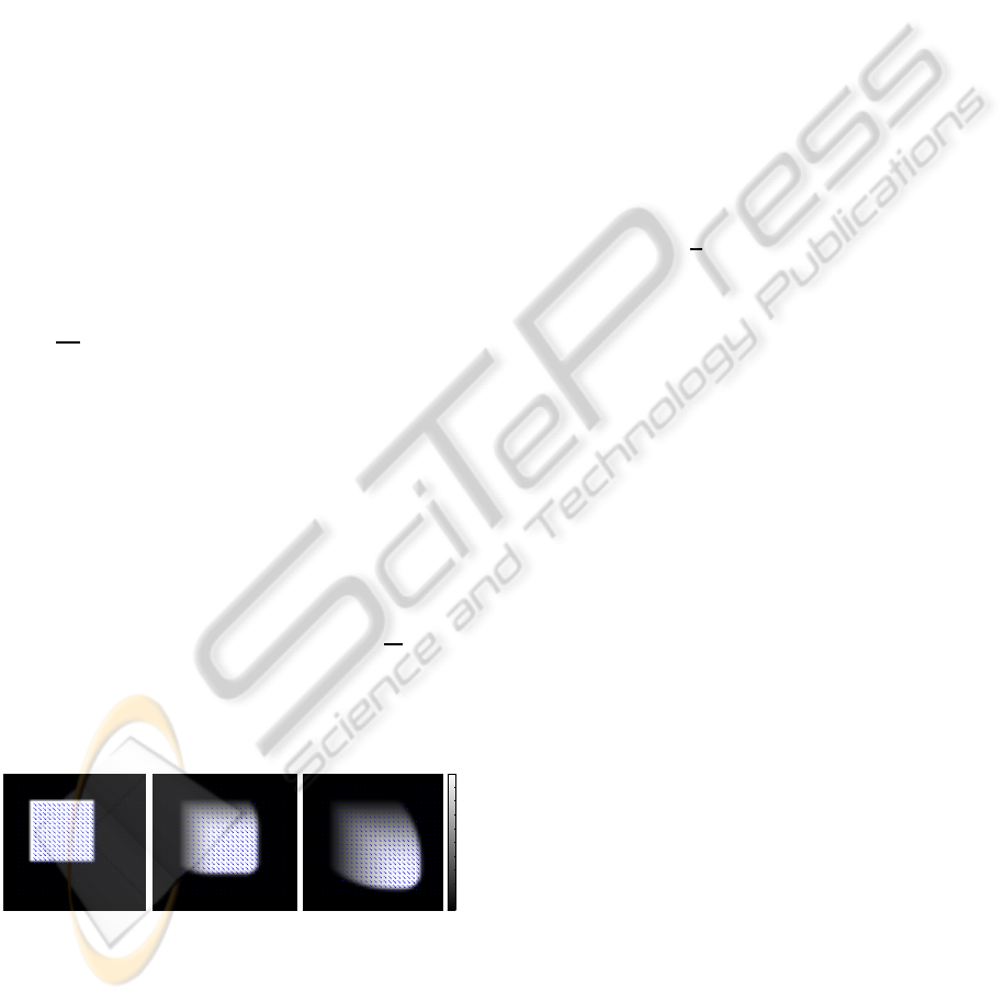
transport process described by (3). See Figure 1 for

an illustration of the transport. We found that our

0.2

0.4

0.6

0.8

1.2

1.4

1.6

1.8

Figure 1: Illustration of the transportation of a vector ﬁeld

with equation (3) at times t = 0,5,10. Gray values visualise

vector magnitudes. Fictive particles move along a shock

front in the lower right direction. In the absence of any

further external information, a region of rarefaction arises

due to mass conservation, acting like a short-time memory.

approach even with the constant velocity assumptions

of our physical prior predicts the non-uniform motion

pattern quite well as shown in our numerical results

(cf. Sec. 4.2).

2.1 Optimal Control Formulation

In the following sections we explain our optimal con-

trol approach. Foundations exploiting ﬂuid dynami-

cal methods can be found in the book of Gunzburger

(Gunzburger, 2002).

We obtain our spatial-temporal control approach

as follows: Additionally to the smoothness term we

introduce a control f, that is distributed in space and

time, which means that it acts over the entire optical

ﬂow domain Ω× [0,T]. The magnitude of the control

is bounded due to penalisation within the objective

functional. The resulting optimisation problem is to

minimise

E(u, f) =

Ω×[0,T]

(∂

I + u· ∇I)

(4)

+ α(|∇u

+ |∇u

) + β| f|

dxdt,

subject to the equations of motion



∂

u+ (u · ∇)u = f in (0,T) × Ω,

∂

u = 0 on (0,T) × Γ.

(5)

We intend to ﬁnd an optimal state u = (u

)

⊤

and an optimal control f = ( f

, f

)

⊤

, such that the

functional E(u, f) is minimised and u and f satisfy

the Burgers equation (5).

The objective of this formulation is to determine

a body force f (the control !) that leads to a velocity

ﬁeld u which ﬁts to the apparent motion in the image

sequence, and at the same time satisﬁes physical prior

knowledge in terms of the given equations of motion.

2.2 Optimality System

In order to obtain the velocity ﬁeld u and the con-

trol f we recast the constrained optimisation problem

(4) - (5) into an unconstrained optimisation problem.

Introducing the Lagrange multiplier or adjoint vari-

able w = (w

(x,t),w

(x,t))

⊤

yields the following La-

grangian functional

L(u, f,w) = E(u, f) (6)

−

Ω×[0,T]

⊤

(∂

u+ (u · ∇)u− f) dxdt.

To solve this functional we have to derive the ﬁrst-

order necessary conditions. This results in the follow-

ing optimality system (7)-(9) from which the optimal

ICINCO 2010 - 7th International Conference on Informatics in Control, Automation and Robotics

state u, adjoints w, and the optimal control f can be

determined such that L(u, f,w) is rendered stationary.







∂

u+ (u · ∇)u = f in Ω× [0,T],

∂

u = 0 on Γ× [0,T],

t=0

= u

in Ω,

(7)











−∂

w− (u· ∇)w− w∇· u + (∇U)

⊤

= ∇I(∂

I + u· ∇I) − α∆u in Ω× [0, T],

w = 0 on Γ× [0,T],

t=T

= 0 in Ω,

(8)







βf + w = 0 in Ω × [0,T],

f = 0 on Γ× [0,T],

t=T

= 0 in Ω,

(9)

where (∇U)

⊤

the transposed Jacobian matrix.

The state equation (7) is obtained by derivation of

the Lagrangian functional (6) in the direction of the

Lagrange multiplier, and turns out to be identical to

the Burgers equation (5) itself. The adjoint equation

(8) speciﬁes the ﬁrst-order necessary conditions

with respect to the state variables u. The optimality

condition (9) is the necessary condition that the

gradient of the objective function – with respect to

the control f – vanishes at the optimum. It also

includes the initial and terminal conditions.

The optimality system (7)-(9) is a coupled system

which turns out to be - due to the large number of

unknowns - prohibitively expensive to solve directly,

but can be solved iteratively as described in the next

section.

2.3 Algorithm

We solve the optimality system (7)-(9) using an itera-

tive gradient descent method (with step length adop-

tion) which decouples the state and adjoint compu-

tation. It consists of the iterative solution of the state

and adjoint equation in such a way that the state equa-

tion is computed forward in time with appropriate ini-

tial condition u

and the adjoint equation is computed

backward in time with terminal condition w

t=T

= 0.

The optimality condition is used to update the control

f with the adjoint variable w. The control f is then

used to compute the actual state u. Additionally, the

step length is adjusted ensuring that the actual energy

of the objective functional (4) decreases. Note that we

choose the start value for f to be zero in the very ﬁrst

iteration.

In our pseudo code description of Algorithm 1,

variable s denotes the step-size that is adapted by the

algorithm and ε the threshold which is used to decide

if the relative difference of the energy is small enough

to be seen as converged.

In the initial step of the algorithm the ﬂow ﬁelds

u for all consecutive image frames and the terminal

condition of the adjoint variable for the last frame

t=T

) are set to zero. The ﬁrst step of the iteration

loop solves the adjoint equation (8) for w backwards

in time using the terminal condition on w and the ﬂow

ﬁeld u. Then, the optimality condition (9) is used to

update the control ﬁeld for all frames, allowing the

state equation (8) to be solved for u forward in time

using the new control ﬁeld. The iteration loop contin-

ues until the decline in E is negligible.

Algorithm 1: Gradient algorithm with automatic step-

length selection.

1: set u = 0, ε = 10

−8

, and s := s

(initial step)

2: repeat

3: solve the adjoint equation (8) for w

4: update f: f

= f

m−1

− s(β f

m−1

+ w)

5: solve the state equation (7) for u

6: if E(u, f

) ≥ E(u, f

m−1

) then

7: s := 0.5s

8: GOTO 4

9: else

10: s := 1.5s

11: end if

12: until |E(u, f

) − E(u, f

m−1

)|/|E(u, f

)| < ε

3 NUMERICAL SOLUTION

In this part, we summarised the numerical discreti-

sation methods employed in solving the optimality

system (7)-(9). For more details, we refer to (Colella

and Puckett, 1998).

Discretisation of the State Equation. Within the

numerical implementation of the nonlinear state

system equation (7) we have to cope with over-

and undershoots, with shock formations, with the

compliance of conditions (entropy-, monotony-,

CFL-condition, etc.) and different discretisation

schemes. We use the second-order conservative

Godunov scheme for our implementation. The ﬂuxes

are numerically computed by solving the equations at

pixel edges. The correct behaviour at discontinuities

is obtained by using solutions of the appropriate

Riemann problem.

Discretisation of the Adjoint Equation. The

numerical implementation of the time-dependent

adjoint system (8) in the domain Ω is done by using

a second-order predictor-corrector ﬁnite difference

IMAGE MOTION ESTIMATION USING OPTIMAL FLOW CONTROL

scheme. The basic idea behind this is that all

methods with an accuracy larger than the order one

will produce spurious oscillations in the vicinity of

large gradients, while being second-order accurate

in regions where the solution is smooth. To prevent

such oscillations the slopes of Fromm’s method are

replaced by the slopes of the Van Leers scheme.

The Van Leer scheme detects discontinuities and

modiﬁes its behaviour in such locations accordingly.

The implication of this is that this method retains the

high-order accuracy of Fromm’s scheme in smooth

regions, but near discontinuities the discretised

evolution equation drops to ﬁrst-order accuracy.

4 EXPERIMENTS

In this section we ﬁrst illustrate the control perfor-

mance of our optical ﬂow approach on a real-world

2D image sequence. Secondly, we evaluate the

following motions which violate the incorporated

motion assumption: rotation, translation in combi-

nation with scaling. Finally, we present the results

for noisy image data showing the inﬂuence of the

temporal regularisation in the control approach and

provide a comparison with error measures obtained

by the approach from (Horn and Schunck, 1981) and

the dynamic optical ﬂow approach from (Stahl et al.,

2006).

4.1 Control - Force

We illustrate the control behaviour of our approach

for a real-world 2D image sequence with an unex-

pected motion. The image sequence consists of 10

image frames and shows a moving hand which starts

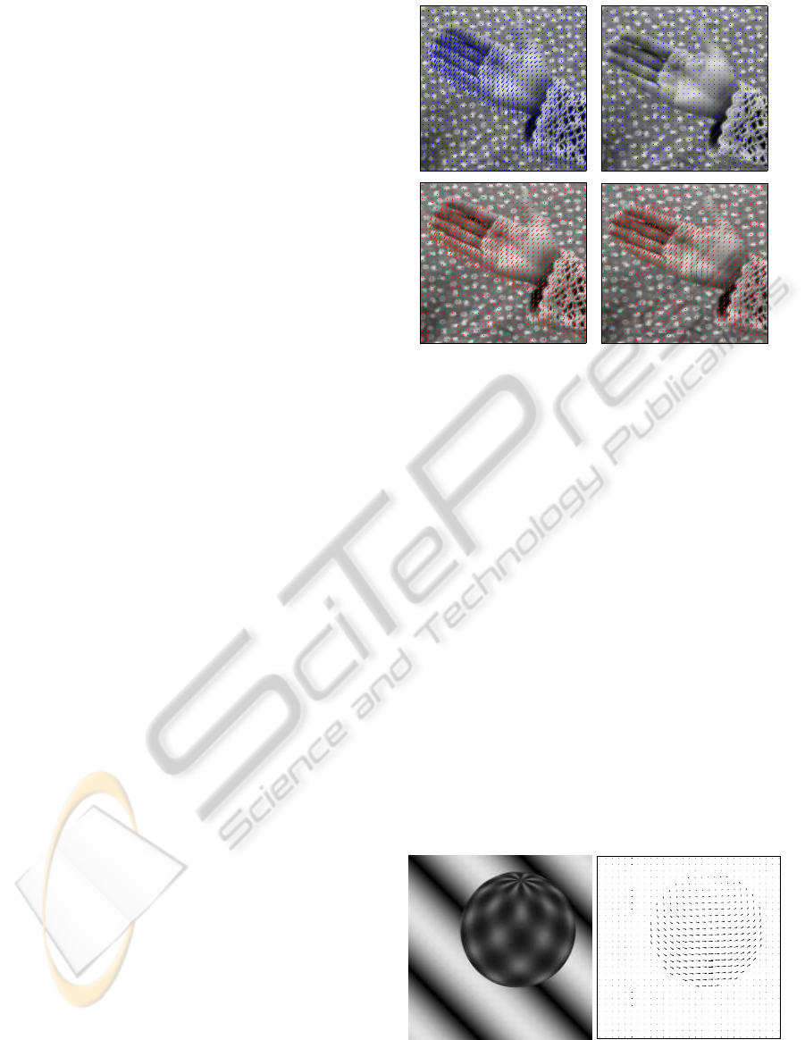
to move and then stops again. Figure 2 depicts the

starting (left column) and stopping (right column)

event of the sequence. The ﬁrst row shows the veloc-

ity estimates u, and the second row shows the force

ﬁelds. The force ﬁeld f nicely indicates the devia-

tion of the expected motion from the observed mo-

tion. This is evident in the second row of Figure 4,

where the force ﬁeld acts in the direction of the mov-

ing hand as the hand accelerates into motion (left pic-

ture), while it turns in the opposite direction as the

hand stops (right picture).

4.2 Non-uniform Motion

In this section we provide an evaluation of our ap-

proach on the basis of two well known synthetic im-

Figure 2: ”Waving hand” sequence: Unexpected events.

Top: A waving hand stops. The estimated optical ﬂow ﬁeld

u for a starting (left) and stopping (right) event is depicted in

blue. Bottom: The corresponding control ﬁeld f is shown

in red. The force acts when the hand starts to move (left)

and reacts into the opposite direction of the ﬂow ﬁeld (right)

when it stops and forces the ﬂow ﬁeld into the observed

state of no motion (parameters: α = 0.01, β = 0.0001).

age sequences for which the ground truth motion data

is available. To allow for a quantitative comparison

we provide the results we obtain for the Horn and

Schunck as well. The image sequences we use show

global motion patterns such as rotation, translation

and divergence.

In particular we evaluate our approach on the

grey value versions of the following two image se-

quences: the ”rotating sphere” sequence (McCane

et al., 2001) and the ”Yosemite” sequence (available

at ftp://ftp.csd.uwo.ca/pub/vision).

The ”rotating sphere” sequence contains a curling

vector ﬁeld and is shown in Figure 3. This sequence

consists of 45 frames, where a sphere rotates in front

of a stationary background.

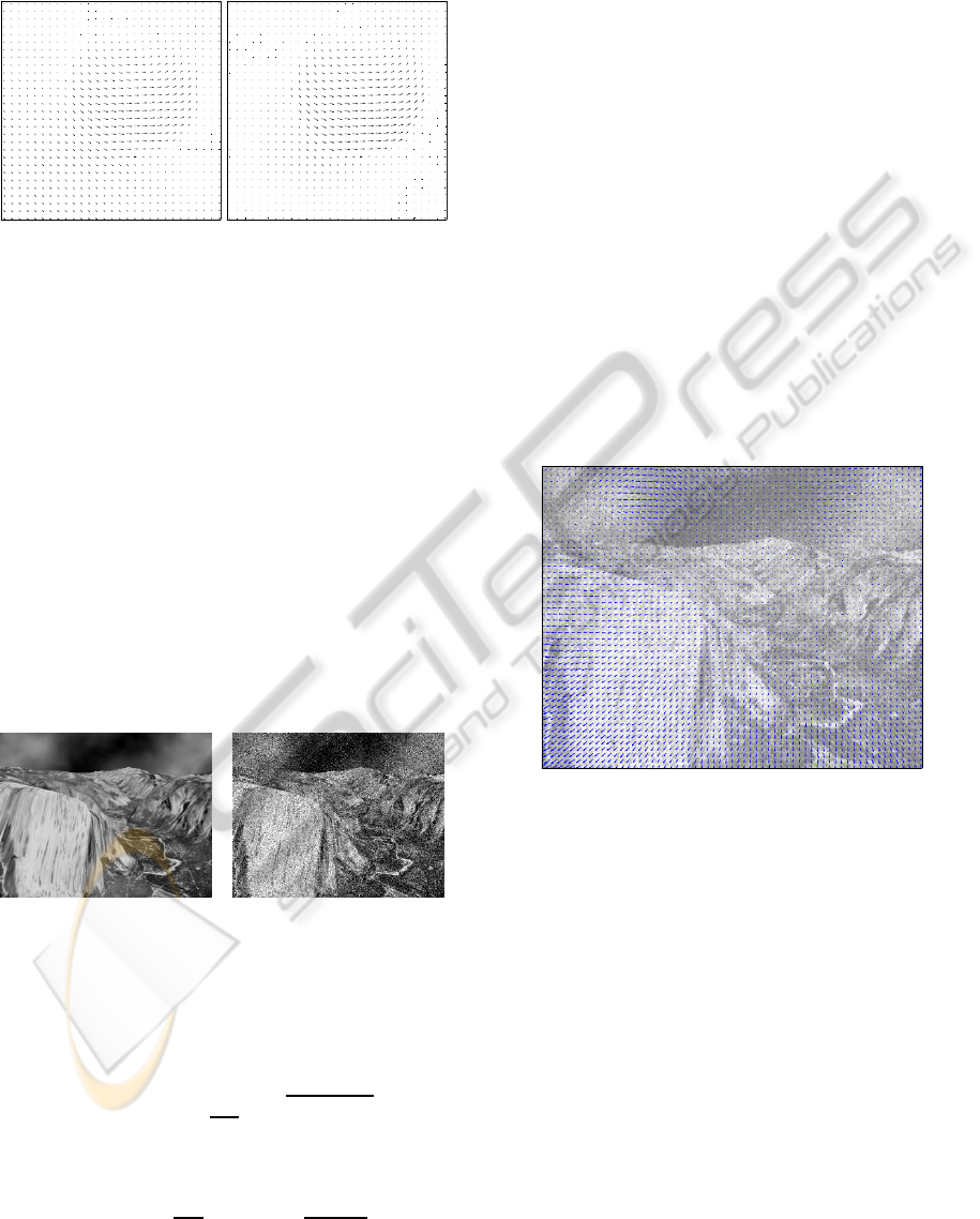
Figure 3: The synthetic ”rotating sphere” sequence. The

sphere rotates in front of a stationary background. Left:

Gray value version of frame 6 that is used in our computa-

tions. Right: Vector plot of the ground truth data.

ICINCO 2010 - 7th International Conference on Informatics in Control, Automation and Robotics

The computed vector ﬁelds obtained by the Horn and

Schunck approach and our approach (4)-(5) for the

”rotating sphere” sequence is shown in Figure 4.

Figure 4: The synthetic ”rotating sphere” sequence. Com-

putational Results for the Horn and Schunck approach and

the control based approach. Left: Result Horn and Schunck

(RMSE = 0.395). Right: Result control based approach

(RMSE = 0.192).

The motion estimation results for the ”Yosemite” se-

quence are shown in section 4.3.

The results show that even for sequences which

violate the constant velocity assumption of the model

equation we obtain good results. However, due to

the ﬂexibility of our variational approach it should be

possible to model such motion patterns by incorpora-

tion of a suitable model equation.

4.3 Temporal Regularisation

To investigate the impact of the temporal regularisa-

tion to the robustness of our approach under noise, we

choose the ”Yosemite” sequence with different Gaus-

sian noise levels σ = 0, 10, 20 and 40 (cf. Fig. 5). The

Figure 5: Top Left: Yosemite sequence. Top Right: We

added Gaussian noise with standard deviation σ = 40.

sequence exhibits divergent and translational motion

combined with illumination changes. To investigate

the performance of our approach we compare the root

mean square error (RMSE)

RMSE(u

) =

|Ω|

Ω

− u

)

and the average angular error (AAE)

AAE(u

) =

|Ω|

Ω

arccos



· u

||u



dx,

where | · | denotes the Euclidean norm, u

,1)

⊤

the original optical ﬂow vectors, and

= (u

,1)

⊤

the estimated optical ﬂow vectors

(compare (Barron et al., 1994)). Note that the time

dimension is set to 1 corresponding to the distance of

one frame.

This measure is currently used as a kind of stan-

dard to provide accuracy measures for optical ﬂow re-

sults.

We compare the errors of the optical ﬂow compu-

tation obtained for three different approaches with op-

timised parameters. In particular these are the homo-

geneous spatial regularised approach from (Horn and

Schunck, 1981), the spatio-temporal dynamic image

motion approach from (Stahl et al., 2006), and our

control based image motion approach (4) - (5). The

control approach results in a improved vector ﬁeld,

which is based on the forward-backward computa-

tion, which incorporates additional knowledge of the

future frames leading to an improved temporal regu-

larisation. The result for a single frame in the highly

noisy Yosemite sequence is shown in Figure 6. The

Figure 6: Temporal regularisation. We added Gaussian

noise with standard derivation σ = 40 to the ”Yosemite”

sequence. The shown high quality optical ﬂow ﬁeld is ob-

tained by the control based optical ﬂow approach (4) - (5)

(parameters: α = 0.05 and β = 0.000003).

results for the computed errors (RMSE and AAE)

for all three approaches with increasing noise level

are shown in Table 1. The purely spatial regularised

approach from Horn and Schunck and the absence

of physical prior knowledge leads to the higher er-

ror values with increasing noise levels. In contrast to

the spatio-temporal dynamic image motion approach

(Stahl et al., 2006) a higher noise level requires the

selection of a smaller β regularisation parameters for

the control part of the objective functional. The con-

sistently lower error indicates an improvedglobal mo-

tion prediction in our control approach (4)-(5) exert-

ing a better temporal regularisation. Our explanation

for this observation is that the control approach incor-

IMAGE MOTION ESTIMATION USING OPTIMAL FLOW CONTROL

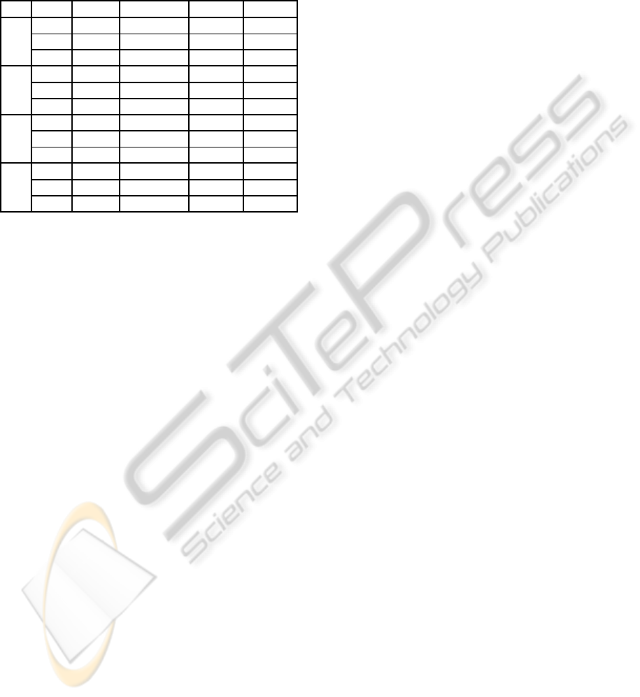
Table 1: Performance of our control approach (C) in com-

parison with the Horn and Schunck approach (HS) and the

dynamic image motion approach (Dy) in presence of noise:

We added random Gaussian noise with zero mean and stan-

dard deviation σ = 0, 10, 20, and 40 to the Yosemite image

sequence.

σ app. α β RMSE AAE

0 HS 0.005 - 0.177 3.04

◦

Dy 0.006 0.00002 0.178 3.09

◦

C 0.007 0.0005 0.169 2.88

◦

10 HS 0.008 - 0.283 5.74

◦

Dy 0.01 0.0003 0.275 5.68

◦

C 0.009 0.0001 0.243 4.92

◦

20 HS 0.02 - 0.429 8.61

◦

Dy 0.025 0.001 0.395 7.54

◦

C 0.02 0.00001 0.350 6.67

◦

40 HS 0.05 - 0.640 13.27

◦

Dy 0.05 0.005 0.523 9.89

◦

C 0.05 0.000003 0.497 9.16

◦

porates also future knowledge of the image sequence

instead of using only past information with a predic-

tion as in (Stahl et al., 2006).

5 CONCLUSIONS

We have presented an optimal control approach to

image motion estimation including physical prior

knowledge in a novel and exploratory way. It leads to

an unconstrainedoptimisation problem, where the op-

timality system - from which the optimal state and the

optimal control are determined - can be solved using

an iterative gradient descent method. The forward-

backward structure of the model allows for a robust

estimation of the coherent ﬂows by including prior

knowledge that enforce spatio-temporal smoothness

of the minimising vector ﬁeld.

In the case that the image measurements indicate

changes of the current velocity distribution, ﬁctive

control forces modify the system state accordingly.

The presence of such forces may serve as an indicator

notifying a higher-level processing stage about unex-

pected motion events in video sequences.

The comparison of our results with the approach

from (Horn and Schunck, 1981) and the approach

from (Stahl et al., 2006) demonstrates the ability of

the control formulation to determine image motion

from video sequences, and shows improved perfor-

mance, especially for highly noisy image data. Our

further work will include the modiﬁcation of the

Burgers equation to achieve better motion boundaries

in the rarefaction area and the reformulation of the

approach to a receding horizon formulation.

ACKNOWLEDGEMENTS

We would like to thank Dr. Christian Schellewald,

Dr. Paul Ruhnau, Prof. Christoph Schn¨orr, and Prof.

Øyvind Stavdahl for some inspiring discussions and

comments.

REFERENCES

Alvarez, L., Esclar`ın, J., Lefebure, M., and S`anchez, J.

(1999). A PDE model for computing the optical ﬂow.

In Proceedings of CEDYA XVI, pages 1349–1356.

Barron, J. L., Fleet, D. J., and Beauchemin, S. S. (1994).

Performance of optical ﬂow techniques. Int. J. of

Computer Vision, 12(1):43–77.

Borzi, A., Ito, K., and Kunisch, K. (2002). Optimal control

formulation for determining optical ﬂow. SIAM J. Sci.

Comput., 24(3):818–847.

Burgers, J. M. (1948). A mathematical model illustrating

the theory of turbulence. Adv. Appl. Mech., 1:171–

199.

Colella, P. and Puckett, E. G. (1998). Modern Nu-

merical Methods for Fluid Flow. Lecture Notes,

Dep. of Mech. Eng., Uni. of California, Berke-

ley, CA. http://www.rzg.mpg.de/ bds/numerics/cfd-

lectures.html.

Deriche, R., Kornprobst, P., and Aubert, G. (1995). Optical-

ﬂow estimation while preserving its discontinuities: A

variational approach. In ACCV, pages 71–80.

Gunzburger, M. (2002). Perspectives in Flow Control

and Optimization. Society for Industrial and Applied

Mathematics.

Hirsch, C. (2000). Numerical Computation of Internal and

External Flows (Vol.I+II). John Wiley & Sons.

Horn, B. and Schunck, B. (1981). Determining optical ﬂow.

Artiﬁcial Intelligence, 17:185–203.

Jain, R., Kasturi, R., and Schunck, B. G. (1995). Machine

Vision. McGraw-Hill, Inc.

Lucas, B. D. and Kanade, T. (1981). An iterative image reg-

istration technique with an application to stereo vision

(darpa). In Proc. of the 1981 DARPA Image Under-

standing Workshop, pages 121–130.

McCane, B., Novins, K., Crannitch, D., and Galvin, B.

(2001). On benchmarking optical ﬂow. Comput. Vis.

Image Underst., 84(1):126–143.

Nagel, H. H. (1990). Extending the ‘oriented smoothness

constraint’ into the temporal domain and the estima-

tion of derivatives of optical ﬂow. In Proc. of the ﬁrst

european conf. on computer vision, pages 139–148.

Springer.

Ruhnau, P. and Schn¨orr, C. (2007). Optical Stokes ﬂow:

An imaging-based control approach. Experiments in

Fluids, 42:61–78.

Schn¨orr, C. (1991). Determining optical ﬂow for irregular

domains by minimizing quadratic functionals of a cer-

tain class. Int. J. of Computer Vision, 6(1):25–38.

ICINCO 2010 - 7th International Conference on Informatics in Control, Automation and Robotics

Stahl, A., Ruhnau, P., and Schn¨orr, C. (2006). A Distributed

Parameter Approach to Dynamic Image Motion. Int.

Workshop on The Representation and Use of Prior

Knowledge in Vision. ECCV Workshop.

Wedel, A., Pock, T., Zach, C., Bischof, H., and Cremers,

D. (2009). An improved algorithm for tv-l1 optical

ﬂow. In Statistical and Geometrical Approaches to

Visual Motion Analysis: International Dagstuhl Semi-

nar, Dagstuhl Castle, Germany, July 13-18, 2008. Re-

vised Papers, pages 23–45. Springer-Verlag.

Weickert, J. and Schn¨orr, C. (2001a). A theoretical frame-

work for convex regularizers in PDE-based compu-

tation of image motion. Int. J. of Computer Vision,

45(3):245–264.

Weickert, J. and Schn¨orr, C. (2001b). Variational optic ﬂow

computation with a spatio-temporal smoothness con-

straint. J. Math. Imaging and Vision, 14(3):245–255.

IMAGE MOTION ESTIMATION USING OPTIMAL FLOW CONTROL