MULTI-SCALE COLLABORATIVE SEARCHING THROUGH
SWARMING
Wangyi Liu, Yasser E. Taima, Martin B. Short and Andrea L. Bertozzi
Department of Mathematics, University of California, Los Angeles, CA 90095-1555, U.S.A.
∗
Keywords:
Mobile robots, Autonomous agents, Searching, Swarming, Target detection.
Abstract:
This paper presents a multi-scale searching and target-locating algorithm for a group of agents moving in a
swarm and sensing potential targets. The aim of the algorithm is to use these agents to efficiently search
for and locate targets with a finite sensing radius in some bounded area. We present an algorithm that both
controls agent movement and analyzes sensor signals to determine where targets are located. We use computer
simulations to determine the effectiveness of this collaborative searching. We derive some physical scaling
properties of the system and compare the results to the data from the simulations.
1 INTRODUCTION
Collaborative sensing has long attracted research in-
terest. Researchers have investigated scenarios where
sensors require localization (Bullo and Cortes, 2005),
where they are used to control collaborative move-
ment (Bopardikar et al., 2007), detect a scalar field
(Gao et al., 2008), or perform a collaborative task
(Smith and Bullo, 2009). Using such collaborating
sensors to detect and locate targets within an area
has been studied in reference to the “mine counter-
measure” problem (Cook et al., 2003), the specific
military task of locating ground or water-based mines.
In this paper, we develop a multi-scale search and
target-locating algorithm for a type of mine counter-
measure problem in which a number of independent
agents are given the task of determining the precise
location of targets within a domain. The algorithm is
designed to handle problems where the scale of the
target sensing radius is much smaller than the domain
size. The focus of this work is to identify optimality
of the algorithm as a function of the swarm size, the
number of agents per group and the distribution of
resources into different groups.
We assume a simply-connected domain, and use
noisy sensors that detect a scalar quantity emitted by
each target, but only when an agent is within a fixed
distance r
s
from a target. We control the motion of
the agents with a model that makes the individuals
∗
This paper is supported by ARO MURI grant 50363-
MA-MUR, ONR grant N000141010641 and NSF grant
DMS-0914856.
form distinct swarms, and present filtering techniques
that allow for locating targets despite noisy data. The
inspiration for this approach comes in part from biol-
ogy, as in the example of birds forming flocks when
flying and searching for food (Travis, 2007).
Next, we analytically derive some of the system’s
main scaling properties, such as the relationship be-
tween swarm size, distance between agents and target
sensing radius, and compare with the experimentally
recorded data. We conclude that our analytical ap-
proach matches well the data from the simulations.
We assume a sensing radius r
s
much smaller than
the domain but comparable to or less than the swarm
size. Other assumptions, however, may require differ-
ent algorithms. For example, in (Burger et al., 2008)
the sensing radius is infinite, but sensing is limited by
obstacles, and in (Olfati-Saber, 2007) communication
between agents is not always possible.
1.1 Scenario Description
We consider M targets in a two-dimensional simply-
connected domain, that is, a flat enclosed area with
no holes, and N agents able to move freely within
the domain. Each target emits a radially symmetric
scalar signal g(r) that decays with the distance r from
the target, and drops to zero at some r
s
, the target’s
sensing radius. Agents detect this signal with an addi-
tional Gaussian, scalar white noise component added.
If an agent is within the sensing radius of multiple tar-
gets, it detects only the sum of the individual signals,
again with a noise component added. We suppose
222
Liu W., E. Taima Y., B. Short M. and L. Bertozzi A. (2010).
MULTI-SCALE COLLABORATIVE SEARCHING THROUGH SWARMING.
In Proceedings of the 7th International Conference on Informatics in Control, Automation and Robotics, pages 222-231
DOI: 10.5220/0002942102220231
Copyright
c
 SciTePress

that an agent takes sensor readings at regular inter-
vals (once per “time step”) spaced such that the noise
between time steps can be assumed independent.
The algorithm accomplishes 3 tasks: it filters the
noisy sensor data, controls the coordinated movement
of the agents based on this data, and determines when
a target has been acquired and where it is located.
1.2 Structure of the Paper
The algorithm is described in the next three sections:
Section 2 focuses on the techniques we use to process
sensor data, Section 3 describes the movement con-
trol of the agents, and Section 4 describes the method
for locating a target. The algorithm is evaluated in
Section 5. Scaling properties are derived and checked
against simulations in Section 6, followed by a con-
clusion and ideas for future research in Section 7.
2 SENSOR DATA PROCESSING
Due to noise in the agent sensor readings and the sens-
ing radius r
s
being finite, we employ two distinct fil-
ters to the data from the readings: a Kalman filter and
a Cumulative Sum (CUSUM) filter. The Kalman filter
reduces or eliminates the noise in the data, while the
CUSUM filter is well-suited to determining whether
or not an agent is within the sensing radius of a target.
The sensor data model follows as a mathematical for-
mula. As explained in Section 1, the formula de-
scribes sensor readings as the sum of scalar signals
that depend only on the distance from a target, to-
gether with a noise component.
Given the M targets at positions y
j
and an agent i with
current position x
i
(t
k
) at timestep k, the agent sensor
reading s
i
(t
k
) is given by
s
i
(t
k
) =
M
∑
j=1
g(|y
j
−x
i
(t
k
)|) + n
i
(t
k
) , (1)
where n
i
(t
k
) denotes sensor noise and g(r) is the sig-
nal strength at a distance r from the target. For sim-
plicity, we assume g(r) is isotropic, smooth, decay-
ing, the same for all targets, and has a cutoff at r
s
.
2.1 Kalman Filtering
Before using the agent sensor readings to locate tar-
gets or control agent motion, we pass the sensor read-
ings through a Kalman filter. Since the signal from
the target is presumed to be varying smoothly with
the distance to the target r (up to the cutoff point r
s
)
as the agents navigate the environment, a Kalman fil-
ter is a natural choice to eliminate or reduce noise in
the sensor readings. The Kalman filter takes the sen-
sor reading s
i
(t
k
) of agent i at time t
k
, and converts it
into the filtered data f
i
(t
k
) according to
P
i
(t
k
) =
P
i
(t
k−1
)R
i
(t
k
)
P
i
(t
k−1
) + R
i
(t
k
)
+ Q
i
(t
k
) , (2)
and
f
i
(t
k
) = f
i
(t
k−1
) +
P
i
(t
k
)(s
i
(t
k
) − f
i
(t
k−1
))
P
i
(t
k
) + R
i
(t
k
)
. (3)
Here R
i
(t
k
) is the square of the noise amplitude,
known or estimated by the agent, and Q
i
(t
k
) is the
square of the change of the signal amplitude between
two time steps, either fixed beforehand or estimated
using the current velocity of the agent (in this paper,
it is fixed beforehand). P
i
(t
k
) is roughly the variance
of the sensor reading’s amplitude. The output f
i
(t
k
) of
this filter is then used in target-locating, as described
in Section 4.
2.2 Threshold Check and the CUSUM
Filter
Before attempting to locate targets, an agent needs to
determine whether or not it is receiving an actual sig-
nal, rather than just noise. In other words, an agent
needs to determine whether it is within the sensing ra-
dius of a target at each time-step t
k
. This information
is then used both in controlling the movement of the
agents and in determining when to begin estimating
a target’s position. In order to determine the sensing
status of an individual agent, we employ a CUSUM
filter, as this type of filter is well-suited to determin-
ing abrupt changes of state (Page, 1954), and has been
used in the similar task of boundary tracking (Jin and
Bertozzi, 2007; Chen et al., 2009). The filter keeps a
sort of running average of the signal and notes when
this average seems to have risen above a cetain thresh-
old, indicating that the agent is now within the sensing
radius of a target. As the noise is effectively summed
up by the filter, it tends to cancel out.
In the original form of the CUSUM filter, we
imagine a sensor that returns a sequence of inde-
pendent observations s(t
1
)...s(t
n
), each of which fol-
lows one of two probability density functions: a pre-
change function g
0
and a post-change function g
1
.
The log-likelihood ratio is
Z(t
k
) = log[g
1
(s(t
k
))/g
0
(s(t
k
))] , (4)
and we define the CUSUM statistic as
U(t
k
) = max(0, Z(t
k
) +U(t
k−1
)), U(t
0
) = 0 . (5)
We then choose a threshold
¯
U, and when U(t
k
) ≥
¯
U
for the first time, the algorithm ends and we declare
MULTI-SCALE COLLABORATIVE SEARCHING THROUGH SWARMING
223

that the state has changed from g
0
to g
1
. The threshold
should be chosen so as to minimize both false-alarms
(these happen more frequently for small
¯
U) and time
to detection (this gets larger as
¯
U increases).
In our system, we choose the special case where
sensor reading follows a Gaussian distribution. In the
pre-change state g
0
, the agent is outside the sensing
radius of any target and reads only noise, which we
model as a Gaussian with zero mean and variance σ
2
.
In the post-change state g
1
, the agent enters the sens-
ing radius of a target, and although the probability dis-
tribution is still a Gaussian with the same variance, the
mean is now larger than zero, which we set to be 2B.
Then
Z(t
k
) = log
"
e
−[s(t
k
)−2B]
2
/2σ
2
/(σ
√
2π)
e
−s(t
k
)
2
/2σ
2
/(σ
√
2π)
#
=
−[s(t
k
) −2B]
2
2σ
2
+
s(t
k
)
2
2σ
2
=
2B
σ
2
[s(t
k
) −B] . (6)
We also modify the algorithm so that it can detect
status changes both into and out of detection zones.
Thus, we implement two filter values: U
i
(t
k
) to deter-
mine when an agent has entered a zone, and L
i
(t
k
) to
determine if it has left a zone. We also define a binary
function b
i
(t
k
) which denotes the status of an agent:
b
i
(t
k
) = 1 means that the agent is near a target and
b
i
(t
k
) = 0 means otherwise. The filter values all start
at zero, and are thus updated according to
U
i
(t
k
) = max(0, s
i
(t
k
) −B +U
i
(t
k−1
)) , (7)
L
i
(t
k
) = min(0, s
i
(t
k
) −B + L
i
(t
k−1
)) , (8)
and
b
i
(t
k
) =



1 b
i
(t
k−1
) = 0, U
i
(t
k
) >
¯
U
0 b
i
(t
k−1
) = 1, L
i
(t
k
) <
¯
L
b
i
(t
k−1
) otherwise.
(9)
In addition, when the status of agent i changes, we re-
set the corresponding U
i
or L
i
to zero. Lastly, we have
set the constant coefficient
2B
σ
2
= 1 for convenience.
Recall that B is a sensor value that is less than the
predicted mean when inside a sensing radius, and
¯
U
is our chosen detection threshold. So, when the agent
is near a target, the sensor reading s
i
(t
k
) tends to be
larger than B, causing U
i
(t
k
) to grow quickly until it
is larger than
¯
U, indicating a change in status. The
converse is true if an agent leaves the sensing region
of a target. The values of filter parameters,
¯
U,
¯
L and
B are problem-specific, and should be set in a manner
that minimizes false-alarms while keeping the aver-
age time to detection as low as possible, as mentioned
above.
Figure 1: Example filter output for an agent as a function of
time, from one of our simulations. The densely-dotted line
represents the true signal that ought to be detected by the
agent. The dots are the actual noisy signal detected by the
agent (i.e., the densely-dotted curve plus noise). The thicker
step function is the signal status returned by the CUSUM
filter, and the thinner straight line represents the value B =
0.1. The sparsely-dashed curve is the output of the Kalman
filter when applied to the detected noisy signal.
An example of sensor reading for an agent from
one of our simulations is in Figure 1. The Kalman
filter does a good job of reducing noise, bringing the
sensor readings much closer to the true signal. Near
the middle of the plot, the agent enters into the sens-
ing radius of a target; this is reflected by a transi-
tion within the CUSUM filter from b = 0 to b = 1.
There is, as expected from the behavior of CUSUM,
a slight delay between when the agent actually enters
into the radius and when this transition of b occurs.
After spending some time within the sensing radius,
the estimated target location stabilizes, the agent sub-
tracts the true signal from its measurements (this will
be explained in Section 4), and the agent leaves to find
further targets.
3 AGENT MOVEMENT
CONTROL
We have chosen to control the movement of our
agents by breaking up our total agent population N
into a number of distinct, leaderless “swarms”. This
is done for a variety of reasons. Firstly, it increases
robustness, as any individual swarm member is not
critical to the functioning of the swarm as a whole.
Secondly, since we imagine that any sensor data ac-
quired by readings from the agents is local in space,
a swarm provides a method of extending the effective
sensing zone to the whole swarm. Thirdly, a swarm of
nearby agents may use their combined measurements
to decrease sensor noise. Finally, a swarm provides
the ability to locate targets via triangulation or gradi-
ent methods. Each swarm may search within its des-
ignated region of space if a divide-and-conquer tactic
ICINCO 2010 - 7th International Conference on Informatics in Control, Automation and Robotics
224

Figure 2: A screenshot from the simulation. Four swarms
with eight agents each are used. Three of them are in the
searching phase, and the upper right swarm is in the target-
locating phase. The large circle around each target marks
the sensing radius. Small crosses are already located targets.
is desired, or it may be free to roam over the entire re-
gion. In the following two sections we mainly focus
on the control of movement for one swarm.
Since the agents detect a limited sensing radius,
we choose to employ two different phases of swarm
motion. When there are no targets nearby, the agents
should move through the space as quickly and as ef-
ficiently as possible, performing a simple flocking
movement as legs of a random search. After a sig-
nal is sensed via the CUSUM filter, the agents should
stop, then slowly move around the area, searching
for the exact position of the nearby target. We call
these two phases the searching phase and the target-
locating phase, respectively. For a general idea of the
two types of motion, see Figure 2.
3.1 The Swarming Model
There are a variety of mathematical constructs that
lead to agent swarming (see for example (Justh and
Krishnaprasad, 2004), (Vicsek et al., 1995), and
(Sepulchre et al., 2008). Here we choose a second-
order control algorithm similar to that described in
(D’Orsogna et al., 2006) and (Chuang et al., 2007),
which has been successfully implemented as a control
algorithm for second-order vehicles on real testbeds
(Nguyen et al., 2005; Leung et al., 2007). In this
system, each agent of the swarm is subject to self-
propulsion and drag, and attractive, repulsive, and ve-
locity alignment forces from each of the other agents.
The position x
i
and velocity v
i
of an individual agent i
with mass m
i
in a swarm of N agents are governed by
dx
i
dt
= v
i
, (10)
and
m
i
dv
i
dt
= (α −β|v
i
|
2
)v
i
−
∇U(x
i
) +
N
∑
j=1
C
o
(v
j
−v
i
) , (11)
where
U(x
i
) =
N
∑
j=1
C
r
e
−|x
i
−x
j
|/l
r
−C
a
e
−|x
i
−x
j
|/l
a
. (12)
C
r
and l
r
are the strength and characteristic length of
the repulsive force, respectively, and C
a
and l
a
are
the corresponding values for the attractive force. C
o
is the velocity alignment coefficient, α is the self-
propulsion coefficient and β is for drag. Depending
on these parameters, the swarm can undergo several
complex motions (D’Orsogna et al., 2006), two of
which are flocking and milling, and in some cases
the swarm can alter its motion spontaneously (Kolpas
et al., 2007). For our purposes, we simply set these
parameters to obtain the type of motion desired.
3.2 Searching Phase
In this phase, the agents move together in one di-
rection as a uniformly-spaced group travelling with
a fixed velocity. Since the agents know nothing yet
about the location of targets, a random search is cho-
sen here. Specifically, we use a L
´
evy flight, which
is optimally efficient under random search conditions
(Viswanathan et al., 1999), and is the same movement
that some birds employ while flocking and searching
for food (Travis, 2007). To accomplish this type of
search, we simply command the swarm to turn by a
random angle after flocking for some random amount
of time. For a L
´
evy flight, the time interval ∆t be-
tween two turns follows the heavy-tailed distribution
P(∆t) ∼ ∆t
−µ
, (13)
where µ is a number satisfying 1 < µ < 3. The value
of µ should be chosen optimally according to the sce-
nario in question, as in (Viswanathan et al., 1999). For
destructive searching (where targets, once located, are
no longer considered valid targets), µ should be as
close to 1 as possible. For non-destructive searching
(i.e. located targets remain as valid future targets), the
optimal µ ∼ 2 −1/[ln(λ/r
s
)]
2
, where λ is the mean
distance between targets and r
s
is the sensing radius.
3.3 Target Locating Phase
When enough agents agree that a target is nearby (see
Section 2.2), the target-locating phase begins. This
MULTI-SCALE COLLABORATIVE SEARCHING THROUGH SWARMING
225

minimum number of agents is set by the swarm con-
sensus parameter p, such that the swarm decides to
enter this phase when p% of the agents or more in the
swarm are sensing a target. Once in this phase, we
want the agents to move only towards the target, so we
remove the velocity alignment force (C
o
= 0), disable
self-propulsion (α = 0), and issue a halt command so
that all agents begin target-locating with zero velocity.
In addition, data from agents within the sensing radius
is used to continually estimate the position ¯y of the tar-
get (see Section 4), and the agents in the swarm then
try to move towards it, thus attracting other agents
in the swarm not yet in the sensing radius to move
closer to the target as well. To make the agents move
towards the target, we add another potential in Equa-
tion 12,
U
c
= C
c
(x
i
− ¯y)
2
/2 , (14)
where ¯y is the estimated position of the target, and C
c
is an adjustible parameter. The full control equations
in the target-locating phase therefore become Equa-
tion 10 and
m
i
dv
i
dt
= −β|v
i
|
2
v
i
−∇U(x
i
) , (15)
where
U(x
i
) =
1
2
C
c
(x
i
− ¯y)
2
+
N
∑
j=1
C
r
e
−|x
i
−x
j
|/l
r
−C
a
e
−|x
i
−x
j
|/l
a
. (16)
To show that this system converges to a stationary
swarm centered on the target, we note that the total
energy of the target-locating system,
E =
1
2
N
∑
i=1
m
i
|v
i
|
2
+
N
∑
i=1
U(x
i
) , (17)
serves as a Lyapunov function, so that the collective
tends to minimize it. That is,
˙
E = −β
N
∑
i=1
|v
i
|
4
≤ 0 . (18)
Hence, velocities will eventually reach zero (due
to drag) and the swarm members will spatially re-
order themselves so as to minimize the potential en-
ergy, forming a regular pattern centered at the target
position. This stationary state serves as a spiral sink,
however, so the swarm tends to oscillate about the tar-
get position for some amount of time that depends on
the value of C
c
, with a high C
c
yielding less oscilla-
tion. However, since the potential being minimized
now includes a term that is effectively attracting all
of the agents towards the center of mass, the swarm
will be more compact than it was before the target-
locating potential was added, so too large of a C
c
will
make the swarm smaller than desired. In practice, we
want C
c
just large enough to minimize the oscillations
in space without making the swarm get too compact.
4 LOCATING TARGETS
During the target-locating phase of motion, all agents
of the swarm that are within the sensing radius keep
a common register of all of their positions and signal
readings made since entering the radius (see “Thresh-
old Check”, Section 2.2, above). The agents then
use a least-squares algorithm to give an estimate ¯y of
where the target is located via
¯y = min
y
N
0
∑
k=1
[g(|y −x(t
k
)|) − f (t
k
)]
2
, (19)
where N
0
is the number of sensor readings in the com-
mon register.
Solving this least-squares minimization is
straightforward, but certain assumptions for work-
ability and precision are needed. It is assumed that
the form of g(r) is known by the agents for the
algorithm to work. For certain classes of targets and
scalar fields, we believe this assumption to be fair.
For precisely estimating a target’s position, we also
assume that only one target is within sensing range, or
that target sensing radii do not overlap significantly,
so that one target is much closer to the agents than
any other target. When the sensing radii are small
compared to the average distance between targets,
these assumptions should hold true. If, instead they
prove to be invalid for the particular system at hand,
other methods such as gradient estimation could be
used.
If the estimated position of the target stabilizes, it
is considered to have been located, and the agents reg-
ister the position of the target and return to the search-
ing phase: the model signal g(r) from the registered
target will be subtracted from further sensor readings
so that it is not detected again, a form of destructive
searching. We thus modify Equation 1 to read:
s
i
(t
k
) =
M
∑
j=1
g(|y
j
−x
i
(t
k
)|) + n
i
(t
k
)
−
M
0
∑
j=1
g(|¯y
j
−x
i
(t
k
)|) , (20)
where M
0
is the total number of registered targets.
Note that the positions of these targets may or may
ICINCO 2010 - 7th International Conference on Informatics in Control, Automation and Robotics
226

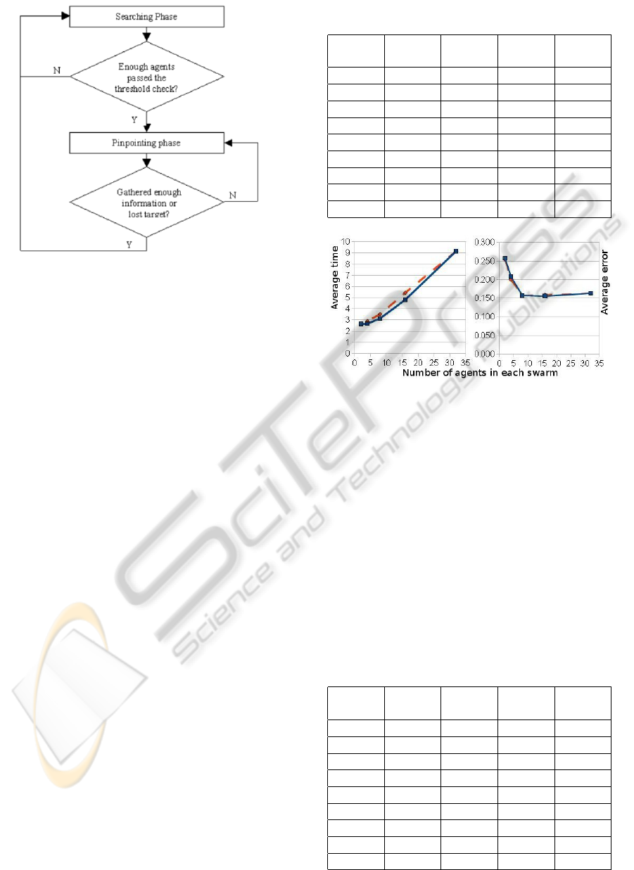
Figure 3: A simple flowchart of the algorithm.
not be accurate, due to noise and other errors. If, in-
stead of the estimated target location stabilizing, the
agents lose track of the target, they simply return to
the searching phase without registering the target. For
a general idea of the entire algorithm, see Figure 3.
5 PERFORMANCE EVALUATION
Two main criteria for the evaluation of this algorithm
are efficiency and accuracy. These are roughly deter-
mined by the two phases: efficiency is mainly related
to the searching phase, while accuracy is mainly re-
lated to the target-locating phase. To evaluate the per-
formance of the algorithm, we divided the agents into
groups and took the following measurements: the av-
erage time needed for a swarm to detect and locate a
target (Average time), the average distance between
the actual and estimated target positions (Average er-
ror), and the percentage of registered positions that
are not within any actual sensing radius (False reg-
isters percentage). Note that false registers are not
included in the average error calculation.
We ran computer simulations of the algorithm in a
dimensionless 20 by 20 area, with a total of 32 agents
and a number of randomly placed targets each with
a dimensionless sensing radius of 1. The signals are
Gaussian (as previously described in Section 2), with
a peak signal-to-noise ratio of about 10.5 dB. Two
cases were considered. In the first case, there were 20
targets and we restricted the duration of the simula-
tion, the main goal being that of measuring efficiency.
In the second case, we distributed just 5 targets ran-
domly, and used a much longer time limit, with the
main goal of measuring accuracy. In both cases, the
Table 1: Case 1: 20 targets, time limit 50.0. Asterisks de-
note the use of the divide-and-conquer tactic.
Swarms Agents/
swarm
Average
time
Average
error
False
reg.
1 32 9.17 0.163 9.77%
2* 16 4.83 0.155 8.40%
2 16 5.45 0.159 11.90%
4* 8 3.15 0.158 8.68%
4 8 3.52 0.16 10.59%
8* 4 2.67 0.208 9.91%
8 4 2.9 0.200 11.73%
16* 2 2.64 0.257 15.59%
16 2 2.64 0.253 15.17%
Figure 4: Average detection time (left) and average error
(right) as a function of the number of agents in each swarm
for case 1 (20 targets and time limit 50.0). The continuous
line is for the divide-and-conquer tactic and the dashed line
is for the results without divide-and-conquer.
simulation ends either when time runs out or when all
targets are found. For each case, we performed 100
trials and calculated the average of the measurements.
Since we considered multiple groups of agents,
it was important to decide how they must cooperate
with one another. We tried two different policies. One
was a simple divide-and-conquer tactic where we di-
vide the whole region into sub-regions before the sim-
ulation, with each swarm in charge of a single sub-
region (Enright et al., 2005; Hsieh et al., 2006), re-
Table 2: Case 2: 5 targets, time limit 200.0. Asterisks de-
note the use of the divide-and-conquer tactic.
Swarms Agents/
swarm
Average
time
Average
error
False
reg.
1 32 45.53 0.128 10.76%
2* 16 25.51 0.116 8.06%
2 16 26.89 0.117 8.95%
4* 8 14.22 0.134 8.96%
4 8 16.64 0.118 8.79%
8* 4 8.35 0.161 7.24%
8 4 10.58 0.172 8.97%
16* 2 8.31 0.223 11.97%
16 2 8.91 0.252 13.79%
MULTI-SCALE COLLABORATIVE SEARCHING THROUGH SWARMING
227

Figure 5: Average detection time (left) and average error
(right) as a function of the number of agents in each swarm
for case 2 (5 targets and time limit 200.0). The continuous
line is for the divide-and-conquer tactic, and the dashed line
is the for the results without divide-and-conquer.
maining within that area the entire time, and perform-
ing a L
´
evy flight search pattern confined to its des-
ignated area. The other policy allows the swarms to
search the entire region independently of one another.
In the results, we denoted the use of the divide-and-
conquer tactic with an asterisk (*).
An important factor that influenced our results
is the number of groups into which we divided the
agents, or equivalently, the number of agents in each
swarm. We therefore present the results for several
choices of this number. They are in Tables 1 and 2,
with the associated plots presented in Figs. 4 and 5.
From the tables and their corresponding plots we
see that the number of agents in the swarm works as
a balance between accuracy and efficiency. As could
have been anticipated, larger swarms give more ac-
curate results (smaller target position error, less false
registers), while multiple, smaller swarms make the
search more efficient (shorter detection time). To
have an acceptably low error and low false register
percentage, groups of at least four agents should be
used. This is perhaps due to the fact that at least three
agents are needed to locate a target, using triangula-
tion. Also, we note that the divide-and-conquer tactic
seems to work somewhat better for this scenario.
6 SCALING PROPERTIES
Having noted the results above, one may wonder how
these are affected by the various scales present in
the system, such as the swarm size, distance between
agents, target sensing radius, etc. Below we present
some arguments for determining optimal search pa-
rameters given these scales.
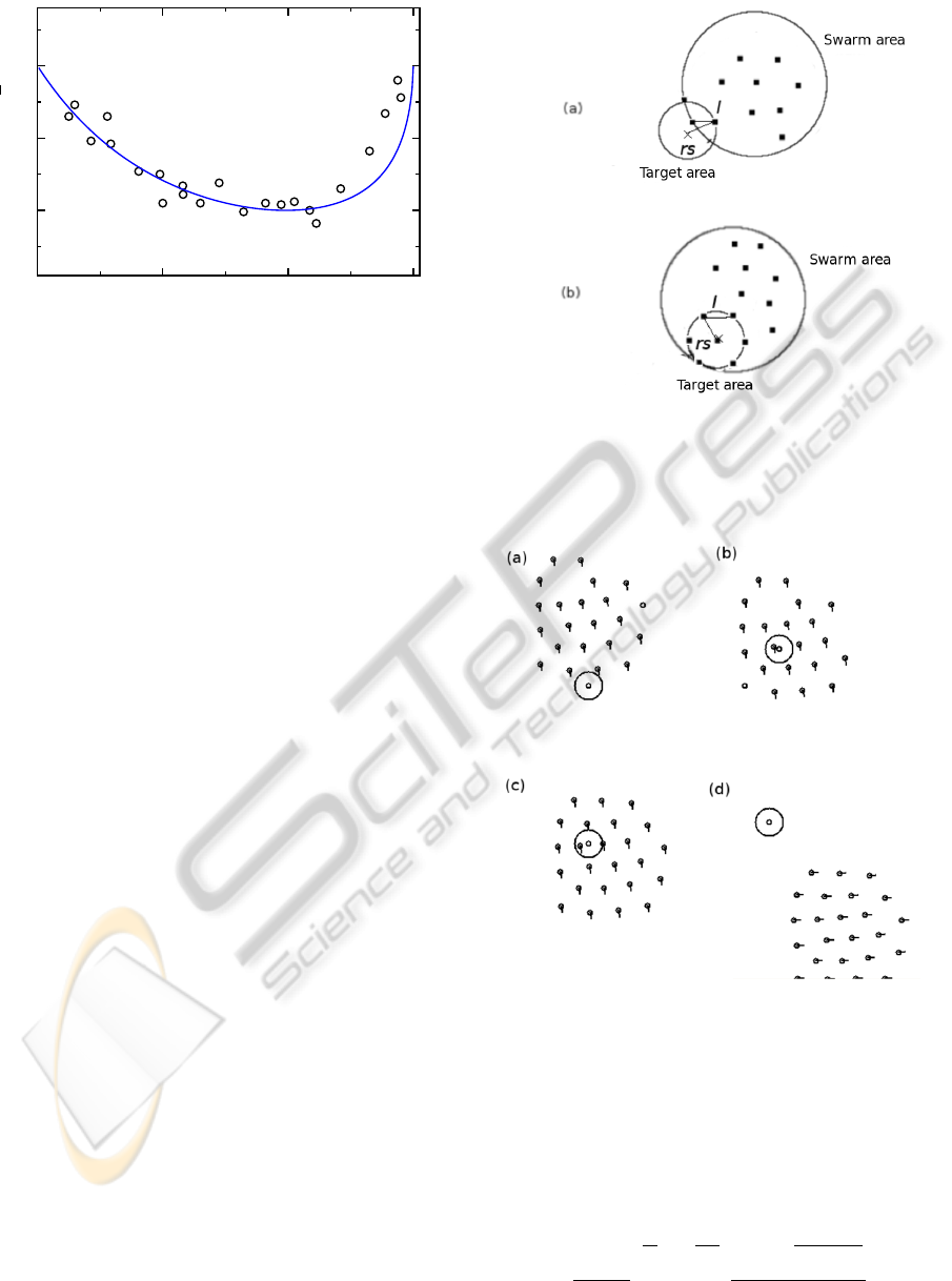
Figure 6: Scales influencing target-locating time: the swarm
diameter D, inter-agent length l, and sensing radius r
s
.
6.1 Estimating the Swarm Diameter
We first define a measure for the swarm size, the
swarm diameter D = max(|x
i
−x
j
|)
N
i=1
, where N is
the number of agents in the swarm. Let us also de-
fine the inter-agent distance l = |x
i
−x
j
| for any two
nearest-neighbor agents i and j (see Figure 6).
For the remainder of this section (and for the re-
sults in Figure 7), we choose the parameters of mo-
tion so that the system is either in regime VI (catas-
trophic) or VII (H-stable) as defined in (D’Orsogna
et al., 2006), with the swarms flocking naturally in
VII, and in VI due to the velocity alignment term C
o
in Equation 11. Under these regimes, D and l sta-
bilize after a transient period, so for the purposes of
this section we will consider them to be constant in
time. In such a stable swarm, agents are uniformly
distributed in space, so that the swarm diameter D
and inter-agent length l are related geometrically as
follows: since the area occupied by a single agent in
the swarm is A
a
≈ πl
2
/4 and the total swarm area is
A
s
= πD
2
/4 ≈ NA
a
, then
D '
√
Nl . (21)
Thus, D scales with l, and for N = 16 (as used in
Figure 7) we get D ' 4l. Since l is approximately the
distance which minimizes the inter-agent potential of
Equation 12, we can easily adjust the swarm diameter
D by varying the system parameters.
6.2 An Upper Bound on the Optimal
Swarm Diameter
Consider a setting with one target of sensing radius r
s
and one swarm of diameter D, as in Figure 6. We
measure the average time to locate the target
¯
T by
starting the swarm at the center of the search field at
time t
0
, placing the target at a random location within
the field, allowing the simulation to run until time T
ICINCO 2010 - 7th International Conference on Informatics in Control, Automation and Robotics
228

0
4
8
12
Swarm diameter, D
150 200 250
Average time,
T
Figure 7: Average time to reach a target
¯
T as a function
of the swarm diameter D for r
s
= 3.0. Values of D were
obtained over a range C
r
= 2.0 −12.0, l
r
= 0.2 −0.7, with
C
a
= l
a
= 1.0. Averaging was carried out over 200 sim-
ulated trials, yielding the numerical results (circles); the
theoretical results of Equation 26 with the best fitting τ
are shown as a line. The number of agents N = 16, and
D
opt
≈ 8.
when the target is found, and averaging these T val-
ues over many runs of the simulation. As D grows, we
observe (see Figure 7) that
¯
T decreases until an opti-
mal swarm diameter D
opt
is reached, after which
¯
T
increases again, growing without bound. We wish to
explain this, first by finding an upper bound on D
opt
.
Let us begin by fixing the swarm consensus per-
centage at p = 25%; i.e., the swarm of agents decides
a target is present when 1/4 of the agents or more are
within the sensing area of a target, A
t
= πr
2
s
(see Fig-
ure 8). Clearly, the borderline case between detection
and non-detection occurs when the target area is com-
pletely subsumed within the swarm area, yet there are
only just enough agents (25% of the total) within the
target sensing radius to detect it. If we assume a con-
stant density of agents in the swarm, this means that
we have detection when the target area is at least p%
= 1/4 of the swarm area. So, it must be the case that
D ≤ 4r
s
, (22)
or else the target will not be detected at all. This con-
dition therefore gives an upper bound on D
opt
. Con-
dition (22) can also be written in terms of l, so that
l ≤r
s
; the borderline case is illustrated in Figure 8(b).
In Figure 9, snapshots from a simulation show how
the swarm flies over the target without being able to
detect it in a case when condition (22) is violated.
6.3 An Approximation for the Optimal
Swarm Diameter
Now that we have an upper bound on D
opt
, we assume
that condition (22) is met and look for approximate
Figure 8: Sensing configurations for the case when 4 or
more agents are required to sense the target before it can
be detected. (a) Though there is overlap between the swarm
and target, too few agents can sense the target for it to be
detected. (b) The largest inter-agent distance l while still
allowing for detection, l = r
s
.
Figure 9: When r
s
is too small compared to D, the swarm
does not detect the target. Snapshots (a)-(d) show the swarm
flying over the target without locating it. Here N = 24, r
s
=
1.5, required percentage for consensus is p = 25%, and D
stabilizes at ≈ 13.5.
expressions for D
opt
and
¯
T . We note that the area of
overlap A
o
between the target and swarm areas, when
the centers are separated by a distance d, is given by
A
o
= r
2
s
arccos

z
r
s

+
D
2
4
arccos

2(d −z)
D

−
z
q
r
2
s
−z
2
−(d −z)
q
D
2
/4 −(d −z)
2
, (23)
MULTI-SCALE COLLABORATIVE SEARCHING THROUGH SWARMING
229

0
4
8
12
Swarm diameter, D
3 3.2 3.4 3.6 3.8
4
d
max
Figure 10: Parameter d
max
versus D for r
s
= 3.0. Note that
d
max
increases at first, as the growing size of the swarm
allows it to be further away while still easily satisfying (22).
However, after the peak at D
opt
≈8, condition (22) becomes
the limiting factor, requiring greater overlap between the
two areas for detection to occur.
where
z ≡
r
2
s
−D
2
/4 +d
2
2d
. (24)
Equation 23 is valid for |r
s
−D/2|≤d ≤r
s
+D/2.
Now, as above, we require that A
o
be at least equal to
25% of the swarm area in order for the target to be
detected. Thus, we obtain an implicit equation for the
maximum separation d
max
between the center of the
swarm and the target location such that the target is
detected:
A
o
(r
s
,D, d
max
) = πD
2
/16 . (25)
The parameter d
max
will depend therefore upon r
s
and
D. At least in terms of the time spent within the
searching phase of the algorithm, the shortest time
¯
T
until detection ought to occur when, for a given r
s
, D
is chosen such that d
max
is maximized (see Figure 10),
giving the largest effective target size to hit; hence this
D should be D
opt
. Furthermore, we expect a scaling
law such that the time to detection is roughly given by
¯
T ≈ τ

A
field
πd
2
max
−1

, (26)
where τ is a characteristic timescale and A
field
is the
total area of the search field.
We have experimentally verified this scaling, with
experimental results usually quite close to the theoret-
ical values, as illustrated by the example with r
s
= 3.0
in Figure 7. We note that the actual time to detec-
tion is a bit above the theory for D > D
opt
, presum-
ably due to our assumption of constant density in de-
riving Equation 25; that is, (especially for large D)
the area of overlap between target and swarm may
be sufficient, but still not contain at least 25% of the
agents, causing the time to detection to be above that
expected.
7 CONCLUSIONS
We considered a mine counter-measure scenario us-
ing multiple agents that move cooperatively via
swarming. The agents use a variety of signal filters
to determine when they are within sensing range of a
target and to reduce noise for more accurate control
and target position estimation. We explored the pa-
rameter space through simulations, determining opti-
mal values for some of the search parameters. We de-
rived scaling properties of the system, compared the
results with data from the simulations, and found a
good analytical-experimental fit.
There are many openings for future research.
First, we could use alternative methods in some parts
of the algorithm. A potential change is to use a
compressed-sensing method (Cai et al., 2008) instead
of least-squares for estimating a target’s location,
which would enable us to find multiple overlapping
targets at the same time. Another interesting modi-
fication would be to use an anisotropic L
´
evy search,
and take previously covered paths into account. Dif-
ferent scenarios could also be evaluated, which might
lead to different results for accuracy and efficiency,
or even suggest new algorithms. For example, we
could extend the two dimensional problem to 3-D, as
would be the case for underwater targets. Or, per-
haps the model for the detected signal is unknown,
in which case we would employ a different method
to estimate the target positions. Finally, apart from
numerical simulations, we plan to do experiments on
a real testbed, with small robotic vehicles as agents.
This would provide an evaluation of the algorithm in
the presence of real sensor noise, which may not be
entirely Gaussian in nature.
ACKNOWLEDGEMENTS
The authors would like to thank Alex Chen and
Alexander Tartakovsky, whose suggestions on the use
of the CUSUM filter were very helpful.
REFERENCES
Bopardikar, S. D., Bullo, F., and Hespanha, J. P. (2007). A
cooperative homicidal chauffeur game. In IEEE Con-
ference on Decision and Control.
Bullo, F. and Cortes, J. (2005). Adaptive and distributed
coordination algorithms for mobile sensing networks.
In Lecture Notes in Control and Information Sciences.
Springer Verlag.
Burger, M., Landa, Y., Tanushev, N., and Tsai, R. (2008).
Discovering point sources in unknown environments.
ICINCO 2010 - 7th International Conference on Informatics in Control, Automation and Robotics
230

In The 8th International Workshop on the Algorithmic
Foundations of Robotics.
Cai, J., Osher, S., and Shen, Z. (2008). Linearized Bregman
iterations for compressed sensing. In UCLA CAM re-
port 08-06.
Chen, A., Wittman, T., Tartakovsky, A., and Bertozzi, A.
(2009). Image segmentation through efficient bound-
ary sampling. In 8th international conference on Sam-
pling Theory and Applications.
Chuang, Y., Huang, Y., D’Orsogna, M., and Bertozzi, A.
(2007). Multi-vehicle flocking: Scalability of cooper-
ative control algorithms using pairwise potentials. In
IEEE International Conference on Robotics and Au-
tomation.
Cook, B., Marthaler, D., Topaz, C., Bertozzi, A., and Kemp,
M. (2003). Fractional bandwidth reacquisition algo-
rithms for vsw-mcm. In Multi-Robot Systems: From
Swarms to Intelligent Automata, volume 2, pages 77–
86. Kluwer Academic Publishers, Dordrecht.
D’Orsogna, M., Chuang, Y., Bertozzi, A., and Chayes, L.
(2006). Self-propelled particles with soft-core inter-
actions: Patterns, stability and collapse. In Physical
Review Letters, 96(10):104302.
Enright, J., Frazzoli, E., Savla, K. and Bullo, F. (2005). On
Multiple UAV Routing with Stochastic Targets: Per-
formance Bounds and Algorithms. In Proceedings of
the AIAA Conference on Guidance, Navigation, and
Control.
Gao, C., Cortes, J., and Bullo, F. (2008). Notes on averaging
over acyclic digraphs and discrete coverage control. In
IEEE Conference on Decision and Control.
Hsieh, C., Chuang, Y.-L., Huang, Y., Leung, K., Bertozzi,
A., and Frazzoli, E. (2006). An Economical Micro-
Car Testbed for Validation of Cooperative Control
Strategies. In Proceedings of the 2006 American Con-
trol Conference, pages 1446–1451.
Jin, Z. and Bertozzi, A. (2007). Environmental boundary
tracking and estimation using multiple autonomous
vehicles. In Proceedings of the 46th IEEE Conference
on Decision and Control.
Justh, E. and Krishnaprasad, P. (2004). Equilibria and steer-
ing laws for planar formations. In Systems & Control
Letters, 52(1):25–38.
Leung, K., Hsieh, C., Huang, Y., Joshi, A., Voroninski, V.,
and Bertozzi, A. (2007). A second generation micro-
vehicle testbed for cooperative control and sensing
strategie. In Proceedings of the 2007 American Con-
trol Conference.
Kolpas, A., Moehlis, J., and Kevrekidis, I. (2007). Coarse-
grained analysis of stochasticity-induced switching
between collective motion states. In Proceedings of
the National Academy of Sciences USA, 104:5931–
5935.
Nguyen, B., Yao-Ling, C., Tung, D., Chung, H., Zhipu, J.,
Ling, S., Marthaler, D., Bertozzi, A., and Murray, R.
(2005). Virtual attractive-repulsive potentials for co-
operative control of second order dynamic vehicles on
the caltech mvwt. In Proceedings of the American
Control Conference.
Olfati-Saber, R. (2007). Distributed tracking for mobile
sensor networks with information-driven mobility. In
Proceedings of the 2007 American Control Confer-
ence.
Page, E. (1954). Continuous inspection schemes. In
Biometrika, 41(1-2):100–115.
Sepulchre, R., Paley, D., and Leonard, N. (2008). Stabiliza-
tion of planar collective motion with limited commu-
nication. In IEEE Transactions on Automatic Control.
Smith, S. L. and Bullo, F. (2009). The dynamic team form-
ing problem: Throughput and delay for unbiased poli-
cies. In Systems & Control Letters.
Travis, J. (2007). Do wandering albatrosses care about
math? In Science, 318:742–743.
Vicsek, T., Czirok, A., Ben-Jacob, E., Cohen, I., and
Shochet, O. (1995). Novel type of phase transition in
a system of self-driven particles. In Physical Review
Letters, 75:1226–1229.
Viswanathan, G., Buldyrev, S., Havlin, S., da Luzk, M., Ra-
posok, E., and Stanley, E. (1999). Optimizing the suc-
cess of random searches. In Nature, 401(6756):911–
914.
MULTI-SCALE COLLABORATIVE SEARCHING THROUGH SWARMING
231