
PERFORMANCE OF HIGH-LEVEL AND LOW-LEVEL
CONTROL FOR COORDINATION OF MOBILE ROBOTS
Sisdarmanto Adinandra, Jurjen Caarls, Dragan Kostić and Henk Nijmeijer
Dept. of Mechanical Engineering, Eindhoven University of Technology, PO Box 513 5600MB, Eindhoven, The Netherlands
Keywords: Coordinated Control, Non-holonomic Systems, High-level and Low-level Control, Collision Avoidance,
Performance Evaluation.
Abstract: We analyze performance of different strategies for coordinated control of mobile robots. By considering an
environment of a distribution center, the robots should transport goods from place A to place B while
maintaining the desired formation and avoiding collisions. We evaluate performance of two collision
avoidance strategies, namely a high-level and low-level collision avoidance approach, each using different
feedback information and update rate. As performance measure we take into account the time to
accomplish the transportation task and the tracking errors of the robots. Evaluation is done in several
experiments with seven mobile robots.
1 INTRODUCTION
A group of mobile robots can be used to realize
spatially distributed transportation tasks in a
distribution center. When several robots are
employed in a shared environment, then motion
coordination and cooperation between these robots
can be introduced in order to increase robustness in
the execution of their tasks.
Transportation in a distribution center is typically
carried out by means of conveyors. Unfortunately, a
failure in a single conveyor can disable a part of the
transportation. To increase robustness of
transportation, one can introduce redundant
conveyers. This solution requires extra investments
and occupies additional space. An appealing
alternative is to substitute conveyers with mobile
robots (Giuzzo, 2008). Unlike conveyers, the robots
can dynamically alter their trajectories to avoid
obstacles and complete assigned tasks. In addition, if
one robot fails, its task can be delegated to another
one. While engaging a number of mobile robots
simultaneously, efficient robot coordination and
cooperation control strategies are required to achieve
high throughput in transportation of goods without
collisions.
In the distribution center, planning and
scheduling tasks are normally done in a centralized
way. A high-level planning system decides which
customers orders must be executed, together with
the decision on how the tasks must be accomplished,
see e.g. (van den Berg, 1999) and (Gu, et al., 2007).
Whereas this centralized approach can provide the
optimal throughput in the absence of uncertainties, it
can show quite some weaknesses in exceptional
situations, such as when unexpected obstacles
appear or when unknown disturbances start affecting
the robots. In such situations, re-planning must be
accomplished with time limitations that often lead to
transportation plans that are not optimal in terms of
the throughput. A viable alternative to the
centralized approach is to facilitate negotiations
among the robots and the supervisor which assigns
the tasks. Through negotiation, the robots and the
supervisor can dynamically adapt the transportation
plans such as to make them less sensitive to different
types of failures. The result might not have the
optimal throughput, but it will likely bring higher
robustness in comparison with the centralized
approach. The high level coordination can be
solved, for instance, using the holonic approach
(Giret and Botti, 2004), (Moneva, et al., 2009).
Another example of the high-level coordination is
decentralized control of Automated Guided Vehicles
for distribution centers (Farahvash and Boucher,
2004), (Weyns, et al., 2005). In both works, a multi
agent system is proposed for transportation planning,
distribution of tasks, and collision avoidance.
At the layer of low-level control of individual
63
Adinandra S., Caarls J., Kosti
´
c D. and Nijmeijer H. (2010).
PERFORMANCE OF HIGH-LEVEL AND LOW-LEVEL CONTROL FOR COORDINATION OF MOBILE ROBOTS.
In Proceedings of the 7th International Conference on Informatics in Control, Automation and Robotics, pages 63-71
DOI: 10.5220/0002943800630071
Copyright
c
SciTePress
mobile robots, various techniques of robot
coordination and cooperation can be used to realize
the transportation, such as leader-follower, behavior
based, virtual structure, etc, (Ren and Beard, 2004),
(Mastellone, et al., 2008), (Sun et al., 2009), (van
den Broek et al., 2009). In these approaches, the
motion controllers achieve tracking of individual
robot trajectories, on the one hand, and maintain the
desired spatial formation between the robots, on
another.
To the best of our knowledge, little research is
devoted to performance comparison between the
high-level and low-level control techniques. Some
research have been conducted on performance
comparison of different high-level techniques, see
e.g. (Vis, 2004), (Le-Anh and De Koster, 2006),
(Gu, et al., 2010) and references therein.
Furthermore, a quantitative evaluation of robustness
of high-level control is still lacking, and no data are
reported that illustrate how complicated it can be for
the high-level control to find the optimal solution.
Finally, there is scarce research on appropriate
combination of high- and low-level control that can
handle both effectiveness and robustness at the same
time.
The lack of information has motivated us to
quantitatively compare performance of high-level
and low-level control of a group of mobile robots
that perform a task which resembles coordinated
transportation of goods in a distribution center. An
ideal situation is simulated as a basis for
comparison. We evaluate performance using
relevant indicators, such as time to accomplish the
task and errors in tracking the desired robot
trajectories.
Two main contributions of this paper are: (i)
suboptimal solutions for motion coordination of
mobile robots, namely pure high-level and pure low-
level coordination and (ii) experimental performance
evaluation of these two strategies for completing
transportation tasks in distribution center like
environments.
This paper is organized as follows. In Section 2
we present necessary mathematical models and
tools. Section 3 explains strategies to coordinate the
motion of the mobile robots. Section 4 reports on
experimental results and highlights the main
findings of our performance analysis. Conclusions
and discussion on future work are given in Section
5.
2 PRELIMINARIES
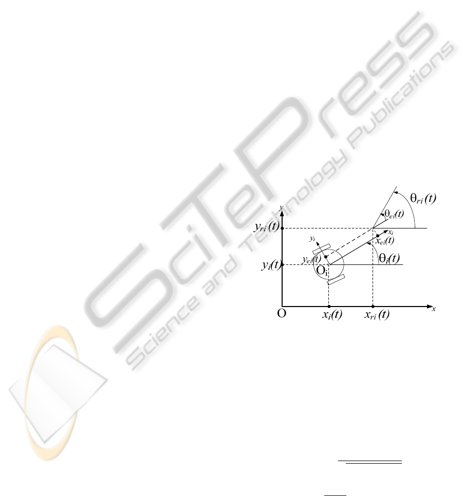
2.1 Unicycle Mobile Robots
We consider a group of m mobile robots that are
described by the non-holonomic kinematic model of
a unicycle, as depicted in Figure 1:
cos
sin
.
(1)
Here,
and
are the forward and steering
velocities, respectively,
and
are the Cartesian
coordinates of the robot midpoint O
i
in the world
coordinate frame O
xy
,
is the heading angle
relative to the x-axis of the world frame, and
∈1,2,3,…,. The reference trajectory of each
robot is given in the frame O
xy
:
.
(2)
The trajectories of all mobile robots constitute a
time-varying formation. An example is shown in
Figure 2, where a platoon-like formation is adopted.
Figure 1: Configuration and error coordinates of a
unicycle mobile robot.
2.2 Trajectory Tracking Control
To follow its own reference trajectory and to
maintain the assigned formation, for each robot we
propose the following control laws v
i
and
ω
i
cos
1
,
,
(3a)
(3b)
ICINCO 2010 - 7th International Conference on Informatics in Control, Automation and Robotics
64

sin
,
sin
1
,
.
where
,
,
are the tracking errors
represented in the robot coordinate frame O
xiyi
cos
sin
0
sin
cos
0
001
,
(3c)
,
,
are the design parameters that influence
the performance of trajectory tracking, while
,
,
are the design parameters that influence
formation keeping. Furthermore,
,∈,, is
defined as follows:
sgn
|
|
sgn
|
|
.
(3d)
The control laws (3a,b) guarantee globally
asymptotic tracking of
and represent a non-
saturated version of the controller proposed in
(Kostić, et al., 2009) and (Kostić, et al., 2010).
Figure 2: An example of a convoy-like, time-varying
formation.
2.3 Penalty Functions
We introduce a set
of continuous, monotone and
bounded penalty functions indexed by a constant
parameter
(Kostić, et al., 2009):
:iscontinous,monotone,
,
i
f
,
,
,
i
f
,
,
i
f
.
(4)
An example of a function in
is
,
,
1Δ
sin
,
,
,
(5)
where Δ
γ
=
-
and = 2π / (
-
).
3 HIGH-LEVEL AND
LOW-LEVEL COORDINATION
To achieve transportation with high throughput and
increase robustness to uncertainties, such as
disturbances, all engaged robots have to cooperate.
These robots have to coordinate their motions such
as to avoid collisions and keep the sequence as
assigned by the given formation.
In this research, we investigate the performance
of two coordination methods, namely high-level
coordination and low-level coordination. The
coordination takes care of collision avoidance and
keeping the desired robot sequence. Both aspects are
very relevant for realization of transportation tasks
in a distribution center environment.
3.1 High-level Coordination
The high-level method of coordination is
implemented at the level of generating the reference
trajectory (2) for each robot. This method assumes
that the robots move from waypoint to waypoint
(nodes) on a network of fixed path segments (edges).
This network enables us to define spatial reference
trajectories.
To accomplish a given transportation task, a
timed desired trajectory along the desired path
segments is generated by each robot. For collision
avoidance it is needed to coordinate (predicted)
intervals of appearance of the robots at intersecting
segments. If these time intervals are well
coordinated, then the absence of collisions is
guaranteed as long as each robot accurately follows
its own reference trajectory. In this case, the
coupling gains
,
and
between robots in the
control laws (3) have to be set to zero. Figure 3
illustrates this coordination method in a situation
where trajectories of three robots intersect at
junction J1.
The junction is represented by a group of
intersecting path segments. Each segment brings a
robot from one side of the junction to another.
Therefore, the interval a robot occupies the junction
PERFORMANCE OF HIGH-LEVEL AND LOW-LEVEL CONTROL FOR COORDINATION OF MOBILE ROBOTS
65
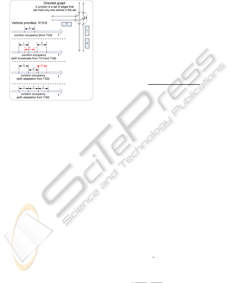
is marked by passing the beginning and ending
waypoints of such a segment.
Figure 3: High-level coordination for collision avoidance.
At regular intervals, currently 1s, each robot
broadcasts its occupation interval to other robots
headed to J1. If overlap is detected, the robot of the
highest priority will rebroadcast its occupation
interval immediately to notify the other robots.
The robot of lower priority will postpone its
arrival time at the junction until the leaving time of
the robot of higher priority. Each robot adjusts its
speed immediately such as to reach the junction at
the correct time. The necessary speed is calculated
and all passing times at the waypoints between the
robot and the junction are adapted accordingly.
Similarly, the passing times after the junction
should be changed too. From the junction segment
on, the passing times are only adapted when the
robot would require to exceed its speed limits. Once
both the entering and leaving waypoint passing
times on the junction are known, the robot
broadcasts its new non-overlapping occupation
interval, and waits again for incoming occupation
intervals.
The priority of a robot is determined as the sum
of the total time this robot has to wait for other ones,
excluding those in front of it, and the expected time
to enter the junction. This is similar to the first come
first served priority scheme, which minimizes the
queues in front of the junctions as well as the
waiting times of the individual robots.
3.2 Low-level Coordination
The low-level coordination is implemented at the
level of trajectory tracking control. To keep the
correct robot sequence according to the desired
spatial pattern, the coupling gain
,
, and
are set to positive non-zero values. With such gains,
the control law (3) will be able to track the desired
formation, e.g. as shown in Figure 2. Due to this
coupling, the robots can recover their formation
faster than their individual desired paths, thereby
maintaining the desired sequence of robots better
than without the coupling.
To gain more robustness to uncertainties, the
reference forward velocity
,
1,2,3,…,
, of
each robot is also adjusted using the penalty
functions from the set
defined by (4). For each
robot we determine the distance between its
reference and actual position:
Δ
,
.
(6)
If Δ
,
, then the desired forward velocity
of each robot i is penalized as follows:
,
Δ
,
.
(7)
Here,
is a penalty function from the set (4)
and
,
is the desired forward velocity. Using (7),
if one robot is far from the assigned path, then the
forward velocities of all robots are decreased in
order to give the perturbed robot time to get back on
its track. In this way, it will be easier to keep the
correct sequence of the robots.
To avoid collisions, we make use of an Artificial
Potential Field (APF) (Latombe, 1991). The
reference trajectories of the robots facing collisions
are online adapted using the APF, mimicking the
approach in (Kostić, et al., 2010). If
,
and
,
, i,j∈ {1,2,...,m}, are the Cartesian
coordinates of the robots i and j, respectively, then
an APF of robot i is:
,
,
,
,
,
(8)
where
,
1
2
,
(9)
,
,
,
0, elsewhere.
.
(10)
ICINCO 2010 - 7th International Conference on Informatics in Control, Automation and Robotics
66
Here, K
o
and K
a
are the gains of the repulsive and
attractive fields, respectively, and are positive
real numbers that determine the size of the detection
region for the repulsive function, rob
d
is the robot
diameter, and d
s
is the threshold of the detection
region. When all obstacles are outside the detection
region of robot i, its tracking controller tracks the
trajectory
. Inside the detection region, the
low-level coordination modifies the trajectory as
follows:
• Determine the Cartesian velocities that move the
robot in the direction of the steepest descent of V
i
(away from the obstruction):
,
,
,
,
,
.
(11)
• Update the reference trajectory such that
collision avoidance is achieved at time-instant t
k
:
,
,
atan
,
/
,
, if
0,
,if
0,
,
,
,
.
(12a)
(12b)
(12c)
(12d)
(12e)
4 EXPERIMENTS AND
PERFORMANCE ANALYSIS
4.1 Scenario
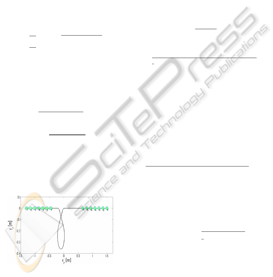
Figure 4: The experimental robot path. Symbols “o” and
“◊” indicate the start and end positions of the robots,
respectively.
To mimic a realistic transportation task in a
distribution center, experiments are conducted
according to the following scenario: a convoy of
seven robots delivers goods along a path depicted in
Figure 4. At one segment of this path, the front part
of the convoy intersects with the part at the back;
consequently, robot coordination is needed to avoid
collisions between the robots and to keep the correct
robot sequence. The desired forward velocity of
each robot is 0.08[m/s].
For performance evaluation, we use the
following indicators:
1. The average of the travel times,
, that the
robots consume to reach their target locations:
∑
,
.
(13)
2. The normalized total tracking error of all robots:
,
∑
∑
,
,
.(14)
where t
k
is the moment of collecting data, l is the
number of data points in the experiment,
,
and
,
are the originally assigned robot reference,
while x
i
and y
i
are the actual positions.
3. The normalized total formation error. In the
experiments we use a platoon-like formation, which
has a spatial pattern described by a time-varying
Euclidean distance between the neighboring robots.
For seven robots, the pattern can be described for
1,2,3,4,5,6 and 1, as follows:
Δ
,
,
,
,
.
(15)
We define the individual formation error by
Δ
Δ
,
(16)
where Δ
is the actual Euclidean distance
between the robots i and j. Thus, the normalized
total formation error is given by:
,
∑∑
1
∑
.
(17)
For a total performance indicator, we take the
summation of the three indicators proposed above
with equal weight:
∑
,
,
.
(18)
4.2 Experimental Set-up
Our experimental setup is depicted in Figure 5. We
PERFORMANCE OF HIGH-LEVEL AND LOW-LEVEL CONTROL FOR COORDINATION OF MOBILE ROBOTS
67
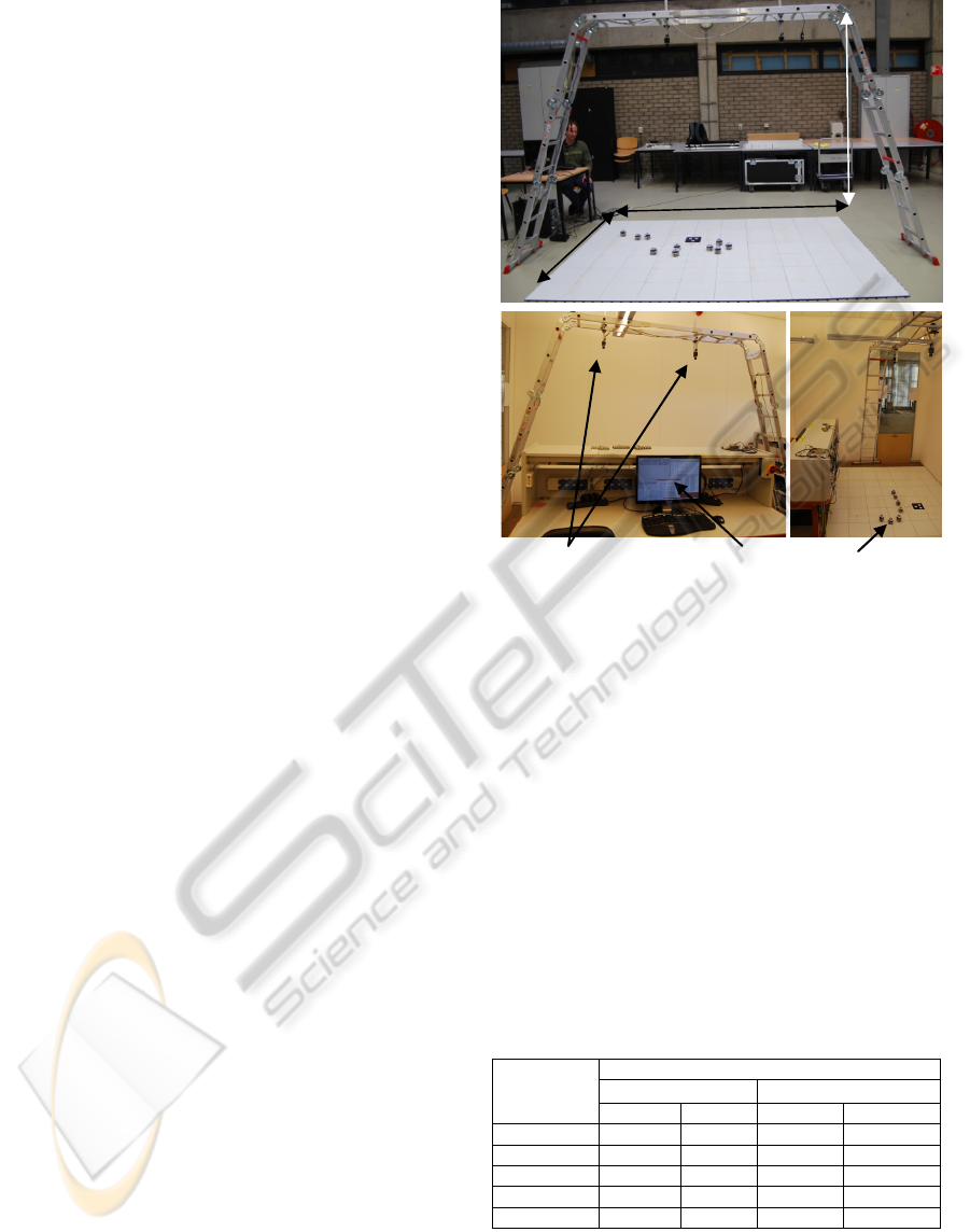
use mobile robots, model e-puck (Mondala and
Bonani, 2007), a camera as a localization device for
getting the position and orientation of all robots, and
a PC. The PC generates robot trajectories, processes
camera images to get the actual pose of the robots,
and runs the collision avoidance algorithms and
tracking control laws for all the robots. The PC
sends the control velocities to the robots via a
BlueTooth protocol. This way of implementation is
chosen due to the limiting processing power of the
onboard robot processors and due to the limited
bandwidth of the BlueTooth communication.
4.3 Experimental Results and Analysis
In the experiments, we use the following design
parameters:
0.4,
100,
0.5,
(19a)
0.06,
10,
0.00001,
(19b)
20,
10,0.05,
(19c)
0.03
m
,
0.14m,
(19d)
0.05
m
,
0.5
m
,
(19e)
,
0.3,
,
1.
(19f)
The values of
,
,
are chosen such that we
have an accurate trajectory tracking. As for
,
,
, the values will be zero if high-level
coordination is active. When low-level coordination
is active, the values are chosen such that we have
strong coupling between the robots, especially in x
and y direction.
As a basis for comparison, we simulate the case
where the coupling terms in the control law (3) are
enabled and collisions are allowed. In this unrealistic
case, all the robots can travel without perturbation
from the start to the end position, while keeping the
formation. To account for realistic imperfections of
the vision system used in experiments, we add
simulated noise, drawn from a normal distribution
with zero mean and standard deviation of ±0.005
[m] for x and y, and ±0.5
0
for
θ
, in accordance with
the measurement noise of the real camera. The
following results are obtained:
36.06
s
,
,
0.0024
m
,
(20a)
,
=0.0019
m
,
∑
36.0643-].
(20b)
Figure 5: The experimental set-up.
The simulation results are used as a reference for
comparison with data obtained from experiments.
Tables 1a and 1b show statistics of all performance
indicators obtained in ten repeated experiments,
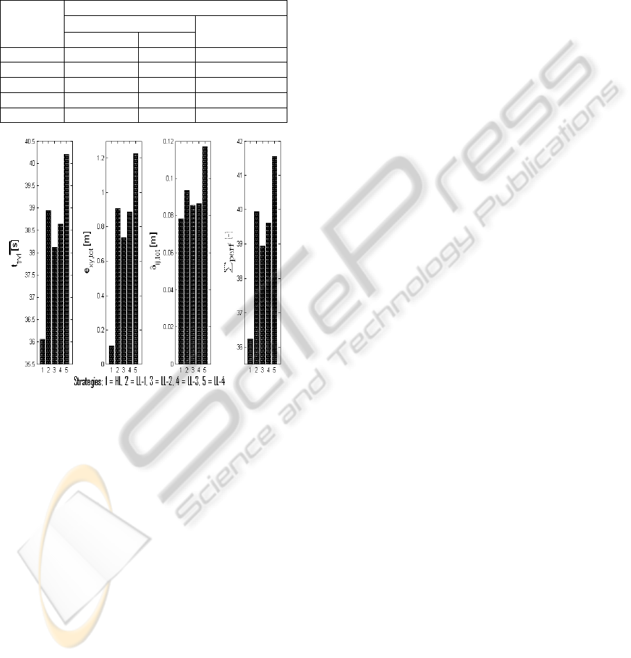
while Figure 6 shows a graphical representation of
these statistics.
ANALYSIS. From the second column of Table 1a
and Figure 6, we can see that the high-level
coordination achieves the shortest average travel
time with respect to other strategies. Thanks to
negotiations among the robots in the high-level
coordination, collision avoidance is achieved time-
efficiently, which leads to short travel times.
Table 1a: Mean value and standard deviation of
and
,
in ten repeated experiments.
Strategies
Indicators
s
,
m
mean Std mean Std
1
HL
36.06
0
0.105 0.00088
2
LL-1 38.939 1.920 0.907 0.4501
3
LL-2 38.110 1.184 0.737 0.3277
4
LL-3 38.633 1.024 0.885 0.2796
5
LL-4 40.204 2.277 1.228 0.3470
1
HL: high-level;
2
LL-1: low level, no coupling between robots
3
LL-2: low-level, all robots are mutually coupled;
4
LL-3: low-
level, each robot is coupled to the leader robot, i.e. the first robot
of the convoy, not vice versa;
5
LL-4: low-level, each robot is
coupled to the robot in front of it, not vice versa.
Two‐camerasystems
PC
E‐pucks
width
hei
g
ht
len
g
th
ICINCO 2010 - 7th International Conference on Informatics in Control, Automation and Robotics
68
Moreover, the travel time is identical to the one
achieved under the ideal condition (20a). The given
experimental result suggests that the high-level
control yields time-optimal transportation while
taking care of collision avoidance.
Table 1b: Mean value and standard deviation of
,
in ten repeated experiments and Σ
perf
.
Strategies
Indicators
,
m
Σ
perf
mean std
1
HL
0.0782
0.00045 36.243200
2
LL-1 0.0934 0.04390 39.939400
3
LL-2 0.0853 0.02390 38.932299
4
LL-3 0.0862 0.00770 39.604199
5
LL-4
0.1170 0.05540 41.548999
Figure 6: The mean values of
,
,
,
,
from
different coordination strategies and Σ
perf
.
As for the low-level coordination, according to
the second column of Table 1a and Figure 6, in all
low-level coordination methods, the total travel time
is longer than achieved using the high-level
coordination. The online APF strategy does not
utilize negotiations; a robot facing an imminent
collision tries to move away from the obstacle.
Time-optimality of such a collision avoidance
algorithm is not guaranteed.
In our experiments, the lowest tracking errors are
achieved using the high-level coordination. With
modest uncertainties, this strategy ensures that each
robot follows its own collision-free reference
trajectory. Consequently, the difference between the
actual and the desired robot trajectories remains
small, which results in small tracking errors. This is
in line with the observation that the shortest travel
time is characteristic for the high level strategy. In
addition, the way the high-level strategy solves the
collision avoidance is also useful for formation
keeping, as depicted in Figure 6.
When comparing the tracking errors, the low-
level coordination strategies, all yield larger tracking
errors compared to the high-level coordination. As
expected, the tracking errors with coupling are
slightly larger than without coupling. Having the
couplings, a robot adapts its movement to other
perturbed robots. In this way, the tracking control
can keep the formation but by doing so, it decrease
its own tracking performance. Despite the poor
tracking error performance, as shown in Figure 6,
introducing correct coupling helps the robots keep
the formation.
If a decision needs to be made, a single measure
is needed to base it on. Comparing the values of the
total performance, we can observe that in our
experiments, option LL-2 turns out to be the most
suitable option for the low-level coordination
method.
Overall, it appears that the high-level control is
the most promising solution according to the total
performance measure. However, this solution may
fail in case of perturbations. The high-level strategy
requires all robots to be in the correct position for a
successful collision-free execution. If one robot is
not at the correct position at some time instant,
collisions may occur and the correct robot
sequencing cannot be guaranteed.
The low-level coordination is inherently more
robust to perturbations. Despite perturbations, the
low-level coordination achieves collision avoidance
and formation keeping. In the presence of
perturbations, from the comparison of the indicators
and considering the importance of formation, the
fully coupled option (LL-2) seems to be the most
appealing one. We show in Table 2 the minimum
distances between the center points of all robots,
measured from an experiment using the LL-2
strategy. During the experiment robot 4 was
manually displaced from the platoon. Since the
diameter of the robot is 0.07 [m], any value below
0.07 [m] implies a collision between robots. Table 2
shows no distances below 0.08 [m], so no collisions
occurred.
Given experimental analysis brings us to the
conclusion that it is not easy to find a single solution
that scores best in terms of all performance
indicators and is robust enough against uncertainties.
There will be a set of solutions that are best, i.e. no
better solutions exist in one performance indicator,
without being worse in another. These solutions are
called pareto-optimal solutions. One has to choose a
PERFORMANCE OF HIGH-LEVEL AND LOW-LEVEL CONTROL FOR COORDINATION OF MOBILE ROBOTS
69

weighing between all indicators, as in the total
performance indicator (18), to select the best one for
a certain application.
Table 2: Minimum distances between the centers of all
robots.
,
denotes the distance between robots i and j.
min
,
[m]
robot 1 2 3 4 5 6 7
1 - 0.08 0.08 0.09 0.16 0.09 0.08
2 - 0.08 0.17 0.23 0.19 0.14
3 - 0.08 0.17 0.20 0.18
4 - 0.08 0.09 0.17
5 - 0.08 0.08
6 - 0.08
The problem remains to find those pareto-
optimal solutions. The high-level and low-level
coordination strategies that we propose still can be
improved and optimized in terms of all performance
indicators, e.g. using larger safety distance for the
high level method or having a smoother transition
from normal to collision mode for the low level
methods. Finding the true pareto-optimal solutions is
probably not possible. However, from a set of
solutions one can always remove the non pareto-
optimal solutions, and choose from the remaining,
best, ones.
5 CONCLUSIONS
We have experimentally evaluated the performance
of different strategies for coordinated control of
mobile robots. We have proposed high-level and
low-level coordination methods and presented
experimental results that illustrate the superior
performance of the high-level method in terms of
time efficiency and accuracy of tracking the desired
robot trajectories. A serious limitation of the high-
level coordination is the requirement for accurate
tracking of the reference trajectories.
Even though the performance of the low-level
coordination method is worse than that of the high-
level coordination method, the low-level one is
inherently more robust against uncertainties.
Given the results of our analysis, it seems
interesting to analyze performance of combinations
of different strategies, e.g., of high-level and low-
level coordination methods. By combining more
strategies, we may optimize more performance
indicators and meet more requirements.
Consequently, it needs to be investigated which
combinations would lead to the pareto-optimal
solutions.
ACKNOWLEDGEMENTS
This work has been carried out as part of the
FALCON project under the responsibility of the
Embedded Systems Institute with Vanderlande
Industries as the industrial partner. This project is
partially supported by the Dutch Ministry of
Economic Affairs under the Embedded Systems
Institute (BSIK03021) program.
REFERENCES
Berg, J. P. van den, 1999, A literature Survey on Planning
and Control of Warehousing Systems, in IIE
Transactions, Vol.31, pp. 751-762.
Broek, T. H. A. van den, van de Wouw, N., Nijmeijer, H.
2009, Formation Control of Unicycle Mobile Robots:
a Virtual Structure Approach, in Proc. IEEE Conf. on
Decision and Control, pp. 8238-8333.
Farahvash, P., and Boucher, T. O., 2004, A Multi-agent
Architecture for Control of AGV Systems, in Robotics
and Computer Integrated Manufacturing, Vol.20, pp.
473-483.
Giret, A., and Botti, V., 2004, Holons and Agents, in J. of
Intelligent Manufacturing, Vol. 15, pp. 645-659.
Giuzzoa, E., 2008, Three Engineers, Hundred of Robots,
One Warehouse, in IEEE Spectrum, Vol. 45. No. 7,
pp. 26-34.
Gu, J., Goetschalckx, M., McGinnis, L. F., 2007, Research
on Warehouse Operation: A Comprehensive review, in
in European Journal of Operational Research, Vol.
177, pp. 1-21.
Gu, J., Goetschalckx, M., McGinnis, L. F., 2010, Reseach
on Warehouse Design and Performance Evaluation: A
Comrehensive review, in European Journal of
Operational Research, Vol. 203, pp. 539-549.
Kostić, D., Adinandra, S., Caarls, J., Nijmeijer, H., 2009,
Collision-free Tracking Control of Unicycle Mobile
Robots, in Proc. IEEE Conf. on Decision and Control,
pp. 5667-5672.
Kostić, D., Adinandra, S., Caarls, J., Nijmeijer, H., 2010,
Collision-free Tracking Control of Unicycle Mobile
Robots, Collision-free Motion Coordination of
Unicycle Multi-agent Systems, Accepted for American
Control Conference 2010.
Latombe, J. C., 1991, Robot Motion Planning, Kluwer
Academic Publishers, Boston, MA.
Le-Anh, De Koster, M. B. M., 2006, A review of Design
and Control of Automated Guided Vehicles Systems,
in European Journal of Operational Research, Vol.
171, pp. 1-23.
Mastellone, S., Stipanović, D. M., Graunke, C. R.,
Intlekofer, K. A., and Spong, M. W., 2008, Formation
Control and Collision Avoidance for Multi-agent Non-
holonomic Systems: Theory and Experiments, in Int.
Journal of Robotics Research, Vol.27, No. 1, pp. 107-
126.
ICINCO 2010 - 7th International Conference on Informatics in Control, Automation and Robotics
70

Mondala, F., Bonani, M., 2007, E-puck education robot,
www.e-puck.org.
Moneva, H., Caarls, J., and Verriet, J., 2009. A Holonic
Approach to Warehouse Control, in Int. Conf. on
Practical Applications of Agents and Multiagent
Systems, pp. 1-10.
Ren, W. and Beard, W., 2004, Decentralized Scheme for
Spacecraft Formation via The Virtual Structure
Approach, in IEEE Proc. Control Theory Application
2004, pp. 268-357.
Sun, D., Wang, C., Shang, W., Feng, G., 2009, A
Synchronization Approach to Trajectory Tracking of
Multiple Mobile Robots While Maintaining Time-
Varying Formations, IEEE Transactions on Robotics,
Vol.25, pp. 1074-1086.
Vis, I. F. A, 2004, Survey of Research in the Design and
Control of Automated Guided Vehicle Systems, in
European Journal of Operational Research, Vol. 170,
pp. 677-709.
Weyns, D., Schelfthout, K., Holvoet, T., and Lefever, T.,
2005, Decentralized Control of E’GV Transportation
Systems, in Autonomous Agents and Multiagent
Systems, Industry Track (Pechoucek, M. and Steiner,
D. and Thompson, S., eds.), pp. 67-74.
PERFORMANCE OF HIGH-LEVEL AND LOW-LEVEL CONTROL FOR COORDINATION OF MOBILE ROBOTS
71
