ARITHMETIC CODING FOR JOINT SOURCE-CHANNEL CODING

Trevor Spiteri and Victor Buttigieg

Department of Communications and Computer Engineering, University of Malta, MSD 2080, Msida, Malta

Keywords:

Arithmetic coding, Joint source-channel coding.

Abstract:

This paper presents a joint source-channel coding technique involving arithmetic coding. The work is based

on an existing maximum a posteriori (MAP) estimation approach in which a forbidden symbol is introduced

into the arithmetic coder to improve error-correction performance. Three improvements to the system are

presented: the placement of the forbidden symbol is modiﬁed to decrease the delay from the introduction of

an error to the detection of the error; the arithmetic decoder is modiﬁed for quicker detection by the introduc-

tion of a look-ahead technique; and the calculation of the MAP metric is modiﬁed for faster error detection.

Experimental results show an improvement of up to 0.4 dB for soft decoding and 0.6 dB for hard decoding.

1 INTRODUCTION

A typical digital communication system includes

source coding and channel coding. Source coding

compresses the data to remove unwanted redundancy

in order to make efﬁcient use of the transmission

channel. Channel coding introduces redundancy in

a controlled manner into the data. This redundancy

can be used by a channel decoder to overcome the ef-

fects of noise and interference in the transmission of

the data, thus increasing the reliability of the system.

Multimedia applications have high data rates so

that compression is a very important part of mul-

timedia systems. Multimedia compression methods

usually include several stages; lossy compression

and quantization techniques are used to remove non-

essential features from the source data, then the quan-

tized data is processed by an entropy encoder. Arith-

metic coding (Rissanen, 1976) is a popular form of

entropy coding. It represents data more compactly

than Huffman coding (Huffman, 1952), and adapts

better to adaptive data models. The use of arithmetic

coding is recently increasing, partly owing to the ex-

piration of key patents that somehowhamperedearlier

adoption.

Data transmission requires both source coding, for

efﬁcient use of the channel, and channel coding, for

reliable data transmission. Joint source-channel cod-

ing techniques are emerging as a good choice to trans-

mit digital data over wireless channels. Shannon’s

source-channel separation theorem suggests that re-

liable data transmission can be accomplished by sep-

arate source and channel coding schemes (Shannon,

1948). Vembu, Verd`u and Steinberg (1995) point out

shortcomings of the separation theorem when dealing

with non-stationary probabilistic channels. The band-

width limitations of the wireless channels, and the

stringent demands of multimedia transmission sys-

tems, are emphasizing the practical shortcomings of

the separation theorem. In practical cases, the source

encoder is not able to remove all the redundancy from

the source. Joint source-channel coding techniques

can exploit this redundancy to improve the reliability

of the transmitted data.

Joint schemes can also provide implementation

advantages. For example, Boyd, Cleary, Irvine,

Rinsma-Melchert and Witten (1997) proposed a joint

source-channel coding technique using arithmetic

codes, and mentioned several advantages, including

(a) saving on software, hardware, or computation time

by having a single engine that performs both source

and channel coding, (b) the ability to control the

amount of redundancy easily to accommodate pre-

vailing channel conditions, and (c) the ability to per-

form error checking continuously as each bit is pro-

cessed.

For error correction, maximum a posteriori

(MAP) decoding (MacKay, 2003) can be used to esti-

mate the transmitted symbols from the received bits.

In MAP decoding, error correction is achieved by

searching for the best path through a decoding tree,

and techniques are required to reduce the complexity

of this tree. In this paper, a MAP decoding scheme by

Grangetto, Cosman and Olmo (2005), which uses a

Spiteri T. and Buttigieg V. (2010).

ARITHMETIC CODING FOR JOINT SOURCE-CHANNEL CODING.

In Proceedings of the International Conference on Signal Processing and Multimedia Applications, pages 5-14

DOI: 10.5220/0002944400050014

 SciTePress

forbidden symbol to detect errors in arithmetic codes,

is described, and novel improvements are presented.

The placement of the forbidden symbol is modiﬁed to

decrease the delay from the introduction of an error

to detection of the error. The arithmetic decoder is

modiﬁed for quicker detection by the introduction of

a look-ahead technique. The calculation of the MAP

metric is also modiﬁed for faster error detection.

Section 2 contains an overview of arithmetic cod-

ing and existing joint source-channel coding tech-

niques based on arithmetic coding, with particular

attention to the maximum a posteriori (MAP) esti-

mation approach by Grangetto et al. (2005). These

schemes have recently received greater attention in

the literature (Bi, Hoffman and Sayood, 2010). Sec-

tion 3 presents novel improvements to the MAP joint

source-channel coding scheme. Section 4 presents ex-

perimental results. Finally, Section 5 draws conclu-

sions.

2 ERROR CORRECTION OF

ARITHMETIC CODES

Arithmetic coding (Rissanen, 1976) is a method for

compressing a message u consisting of a sequence of

L symbols u

, u

, ··· , u

with different probability of

occurrence. Arithmetic coding requires a good source

model which describes the distribution of probabili-

ties for the input symbols. The source model can be

static or adaptive. In a static model, the distribution of

probabilities remains ﬁxed throughout the message,

that is, it is the same when encoding the ﬁrst sym-

bol and when encoding the last symbol. In an adap-

tive model, the probability distribution can be updated

from symbol to symbol, so the probability distribution

used to encode the last symbol may be different from

that used to encode the ﬁrst symbol.

Arithmetic coding can be thought of as represent-

ing a message as a probability interval. At the start

of the encoding process, the interval is the half-open

interval [0, 1), that is, 0 ≤ x < 1. For each sym-

bol u

to be encoded, this interval is split into sub-

intervals with widths proportional to the probability

of each possible symbol, and the sub-interval corre-

sponding to the symbol u

is selected. This interval

gets progressively smaller, so to keep the interval rep-

resentable in computers, it is normalized continuously

(Witten, Neal and Cleary, 1987). When the interval is

small enough, bits are emitted by the encoder and the

interval is expanded.

2.1 Error Detection

Arithmetic coding can compress data optimally when

the source model is accurate. However, arithmetic

codes are extremely vulnerable to any errors that

occur (Lelewer and Hirschberg, 1987). Huffman

codes tend to be self-synchronizing, so errors tend

not to propagate very far; when an error occurs in

a Huffman-coded message, several codewords are

misinterpreted, but before long, the decoder is back

in synchronization with the encoder (Lelewer and

Hirschberg, 1987). Arithmetic coding, on the other

hand, has no ability to withstand errors.

Boyd et al. (1997) propose the introduction of

some redundancy in arithmetic codes. This is done

by forbidding a range from the interval. In common

arithmetic coding techniques, the coding interval is

doubled when required (Witten et al., 1987). Boyd

et al. suggest the interval to be reduced by a factor R

each time the interval is doubled, consequently for-

bidding part of the interval. When this redundancy

is introduced, errors can be detected by the decoder

when the decoding interval falls within a forbidden

part. The delay from the bit error to the detection of

an error is shown to be about 1/(1−R).

Instead of rescaling the interval for every normal-

ization interval doubling, Sayir (1999) suggests in-

troducing forbidden gaps in the interval. After each

source symbol is encoded, the source probabilities are

rescaled by a rescaling factor γ, such that on average,

−log

γ bits of redundancyare added for every source

symbol. The gap factor ε is deﬁned to be ε = 1−γ.

2.2 MAP Decoding

The forbidden gap technique is a joint source-channel

method for detecting errors in arithmetic codes. To

perform error correction, we must ﬁrst encode the

symbols with an encoder that introduces redundancy.

Suppose we have a message u consisting of a se-

quence of L symbols, u

, u

, ··· , u

. We encode this

into a bit sequence t, which has N bits, t

, t

, ··· , t

The bit sequence t is then transmitted over a noisy

channel, and the received signal is y. Figure 1 is a

block diagram of the encoding and decoding process.

The task of the decoder is to infer the message

u given

the received signal y. If the inferred message

u is not

identical to the source message u, a decoding error

has occurred.

Arithmetic

Encoder

Channel

ûy

Arithmetic

Decoder

Figure 1: Block diagram of the encoding and decoding pro-

cess.

SIGMAP 2010 - International Conference on Signal Processing and Multimedia Applications

MAP decoding (MacKay, 2003) is the identiﬁca-

tion of the most probable message u given the re-

ceived signal y. By Bayes’ theorem, the a posteriori

probability of u is

P(u|y) =

P(y|u)P(u)

P(y)

. (1)

Since u has L elements and the signal y has N ele-

ments, it can be convenient to work in terms of the bit

sequence t instead of the message u. Since there is a

one-to-one relationship between u and t, P(t) = P(u).

Thus, we can rewrite (1) as

P(t|y) =

P(y|t)P(t)

P(y)

. (2)

The right-hand side of this equation has three parts.

1. The ﬁrst factor in the numerator, P(y|t) is the

likelihood of the bit sequence t, which is equal to

P(y|u). For a memoryless channel, the likelihood

may be separated into a product of the likelihood

of each bit, that is,

P(y|t) =

∏

n=1

P(y

). (3)

If we transmit +x for t

= 1 and −x for t

= 0

over a Gaussian channel with additive white noise

of standard deviation σ, the probability density of

the received signal y

for both values of t

P(y

= 1) =

√

2π

exp



−

−x)

2σ



(4)

P(y

= 0) =

√

2π

exp



−

+ x)

2σ



. (5)

2. The second factor in the numerator, P(t), is the

prior probability of the bit sequence t. In our case,

this probability is equal to P(u), so that

P(t) =

∏

l=1

P(u

). (6)

3. The denominator is the normalizing constant. The

normalizing constant is the sum of P(y|t)P(t) for

all possible bit sequences t.

P(y) =

∑

P(y|t)P(t) (7)

The normalizing constant has a value such that the

sum of P(t|y) for all possible t becomes 1.

∑

P(t|y) =

∑

P(y|t)P(t)

P(y)

∑

P(y|t)P(t)

P(y)

∑

P(y|t)P(t)

∑

P(y|t)P(t)

= 1

MAP decoding can be summed up as the process

of identifying the message u with the highest proba-

bility P(u|y) giventhe receivedsignal y. So the prob-

lem of decoding arithmetic codes using MAP decod-

ing is a problem of searching for this best u from all

possible sequences u.

To search for the required u, we build a decod-

ing tree. The tree consists of a number of nodes (or

states) and a number of edges connecting them. The

state may be either the bit state or the symbol state.

If we are using the bit state, each edge will represent

one bit, and each node will have two child nodes, one

corresponding to a

, and the other corresponding to

. When traversing this tree, going from one state

to the next (from one node to its child) happens every

time we decode one bit.

If we are using the symbol state, the edges will

represent symbols instead of bits, and the number of

child nodes depends on the number of possible sym-

bols. This time, going from one state to the next hap-

pens every time we decode one symbol.

For arithmetic codes, the size of the decoding tree

increases exponentially with the number of symbols

in the input sequence. So we have to use techniques

to limit our search on some section of the tree; it is not

feasible to compute P(u|y) for all possible sequences

Guionnet and Guillemot (2003) present a scheme

that uses synchronization markers in the arithmetic

codes. They use two kinds of markers: bit mark-

ers and symbol markers. For bit markers, a number

of dummy bit patterns are introduced into the bit se-

quence after encoding a known number of symbols.

The number of bits required to encode a number of

symbols is not ﬁxed, so these bit markers will occur

at random places in the output bit sequence. The de-

coder then expects to ﬁnd these bit patterns when de-

coding, and if the patterns are not found, the path is

pruned from the decoding tree. Alternatively, symbol

markers can be used. Instead of inserting a bit pattern,

a number of dummy symbols are inserted into the in-

put sequence after a known number of input symbols.

As for the bit markers, if the decoder does not ﬁnd

these dummy symbols during decoding, the path is

pruned from the decoding tree.

Grangetto et al. (2005) present another MAP es-

timation approach for error correction of arithmetic

codes. Instead of bit markers or symbol markers, they

use the forbidden gap technique mentioned in Section

2.1. The decoding tree uses the bit state, rather than

the symbol state. Whenever an error is detected in a

path of the decoding tree, that path is pruned. The

number of bits N is sent as side information. If a path

in the tree has N nodes but is not yet fully decoded,

ARITHMETIC CODING FOR JOINT SOURCE-CHANNEL CODING

the detector prunes the path. Grangetto et al. com-

pare this joint source-channel scheme to a separated

scheme. In the separated scheme, an arithmetic code

with ε = 0 is protected by a rate-compatible punc-

tured convolutional (RCPC) code. The RCPC code

used was of the family with memory ν = 6 and non-

punctured rate 1/3, proposed by Hagenauer (1988).

The comparison indicated an improvement over the

separated scheme.

In another paper, Grangetto, Scanavino, Olmo and

Benedetto (2007) present an iterative decoding tech-

nique that uses an adapted BCJR algorithm (Bahl,

Cocke, Jelinek and Raviv, 1974) for error correction

of arithmetic codes.

In this paper, the ideas in Grangetto et al. (2005)

are implemented and some novel improvements are

introduced. Recall that in MAP decoding, the prob-

lem is to ﬁnd the transmitted sequence t which has

the maximum probability P(t|y), and that this proba-

bility can be written as

P(t|y) =

P(y|t)P(t)

P(y)

As shown above, the right-hand side of this equation

has three parts, the likelihood P(y|t), the prior prob-

ability P(t), and the normalizing constant P(y).

The a posteriori probability P(t|y) is the decod-

ing metric used, that is, the decoding algorithm tries

to maximize this value. In the case of memoryless

channels, we can use an additive metric m by taking

logs of the decoding metric.

m = logP(t|y)

m = logP(y|t) + logP(t) −logP(y). (8)

The additive decoding metric m can be split into

N parts,

m =

∑

n=1

(9)

where m

is the part of m corresponding to the nth

bit. This is convenient as it enables us to update the

metric m for each channel symbol y

we try to decode.

That is, after each bit, we can update the metric m.

Combining (8) and (9) gives us

= logP(y

) + logP(t

) −logP(y

). (10)

Notice that the second term on the right-hand side, the

prior probability, is not very straightforward to evalu-

ate. We know that P(t) = P(u), because the transmit-

ted bit sequence t has a one-to-one relationship with

the input symbol sequence u. When decoding a se-

quence y, for each channel symbol, the decoder will

either decode no source symbols, or it will decode one

or more source symbols. Suppose that using bit y

the decoder decodes the symbols u

. u

is a vector

containing I source symbols u

n,1

, u

n,2

, ··· , u

n,I

. If no

symbols are decoded after bit y

, I = 0 and u

is an

empty vector. In any case,

logP(u

) =

∑

i=1

logP(u

n,i

). (11)

We can approximate (10) as

= logP(y

) + logP(u

) −logP(y

). (12)

It is worth pointing out that equations (10) and (12)

are not exactly the same. Since P(t) = P(u), we can

say that

∑

n=1

P(t

) =

∑

n=1

P(u

), but this does not

mean that P(t

) = P(u

The normalizing constant P(y) is difﬁcult to eval-

uate; (7) indicates that this requires knowledge of all

possible bit sequences t, which is not feasible. To

solve this problem, Grangetto et al. (2005) use an ap-

proximation by Park and Miller (2002). The bit se-

quence contains N bits, so assuming that all 2

bit

sequences are possible, then

P(y) ≈

∏

n=1

P(y

= 1) + P(y

= 0)

. (13)

2.2.1 Hard-decision and Soft-decision Decoding

Suppose we have an additive white Gaussian noise

(AWGN) channel using binary phase-shift keying

(BPSK) modulation with a signal-to-noise ratio

For hard-decision decoding the signal y

can be

either 0 or 1. The channel transition probability is

P(y

) =



1− p if y

= t

p if y

6= t

(14)

where p is the probability that a bit is demodulated

in error, p =

erfc

. From (13) and (14) it is

easy to deduce that

P(y

) =

, (15)

so that (12) becomes

= logP(y

) + logP(u

) + log2. (16)

For soft-decision decoding, the metric can be

found in a similar way. As in the case of hard-decision

decoding, suppose we have an AWGN channel using

BPSK modulation with a signal-to-noise ratio E

The signal y

will not be constrained to only two val-

ues, 0 and 1. Recall that the probability distribution

for y

is given by equations (4) and (5). For BPSK

modulation and an AWGN channel, x =

√

and

SIGMAP 2010 - International Conference on Signal Processing and Multimedia Applications

σ =

/2. As we have done for the hard-decision

decoding metric, we can approximate P(y

) by

P(y

) =

P(y

= 1) + P(y

= 0)

Using this approximation, from (4) and (5) we can

ﬁnd that

P(y

= 1)

P(y

)

2exp



√



exp



√



+ 1

(17)

P(y

= 0)

P(y

)

exp



√



+ 1

. (18)

Substituting (17) and (18) into (12) gives us











logP(u

) + log2+



√



−log

exp



√



+ 1

if t

= 1

logP(u

) + log2

−log

exp



√



+ 1

if t

= 0.

(19)

2.3 Stack Algorithm

Direct evaluation of the MAP metric over all possible

bit sequences is not feasible. The size of the decod-

ing tree would grow exponentially with the number of

symbols L. To prevent this problem, sequential search

techniques are used.

The decoder proposed by Grangetto et al. (2005)

uses a search algorithm along the branches of a binary

tree. The sequential algorithm used is the stack algo-

rithm (Jelinek, 1969). The tree paths are kept in a list

ordered by their metric; the path with the best metric

is kept at the top of the list.

In each iteration, the best path is removedfrom the

list and replaced by two paths; one assuming t

= 0,

and the other assuming t

= 1. These two new paths

then have their corresponding metrics updated, and

are suitably placed in the ordered list.

The ordered list has a predeﬁned maximum size

M. When there are more then M paths, the paths with

the worst metric are removed from the list.

Although the algorithm is called a stack algorithm,

because the concept of a stack is useful for describing

the algorithm, Jelinek (1969) suggests that storing the

paths in a physical stack is not optimal, and that it is

preferable to store the paths in random access storage.

A physical stack would require a sequential compar-

ison of the metric to insert a path, and relocation of

large amounts of data in the required stack position.

As an alternative method, Jelinek proposes splitting

the stack into a number of buckets, each containing

metrics that are close in value.

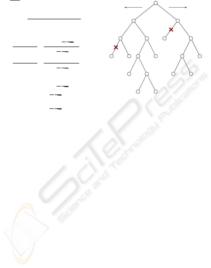
0 1

2.1 1.6

1.9 3.8 0.2 1.1

0.4 2.2 0.4 3.5 2.1

0.3 1.2 2.9 4.7

0.8 0.9

1 2

121143

9 10 5 6 15 16

18178

13 14

Figure 2: Example binary decoding tree.

Figure 2 shows an example decoding tree as it

evolves during the decoding process. At the start of

the process, there is only one node, node 0, with met-

ric m

= 0. In each step, the node with the highest

metric is split into two nodes, the node to the left

assuming t

= 0 and the node to the right assuming

= 1. Sometimes a path is pruned because one of

two conditions occurs: either (a) the decoder detects

an error in the path, or (b) the number of nodes in the

tree exceeds the limit M, so the worst path is removed

from the tree.

3 IMPROVED ERROR CONTROL

The MAP decoding scheme presented by Grangetto et

al. (2005) was implemented and some novel improve-

ments were introduced. To enable a fair comparison,

the data encoded during testing is of the same form as

that used by Grangetto et al.

3.1 Placing the Forbidden Gap

We have already seen that a forbidden gap can be used

to detect errors in arithmetic codes. In Sayir (1999),

the gap is placed at the end of the interval. Placing

the gap at a different location may reduce the error-

detection delay.

To investigate this possibility, an arithmetic coder

was used on a binary source with symbols a and b,

with probabilities P(a) and P(b). Experimental re-

sults indicate that, when using the look-ahead tech-

nique presented in Section 3.2 below, if P(a) > P(b),

the forbidden gap should be placed before the sym-

ARITHMETIC CODING FOR JOINT SOURCE-CHANNEL CODING

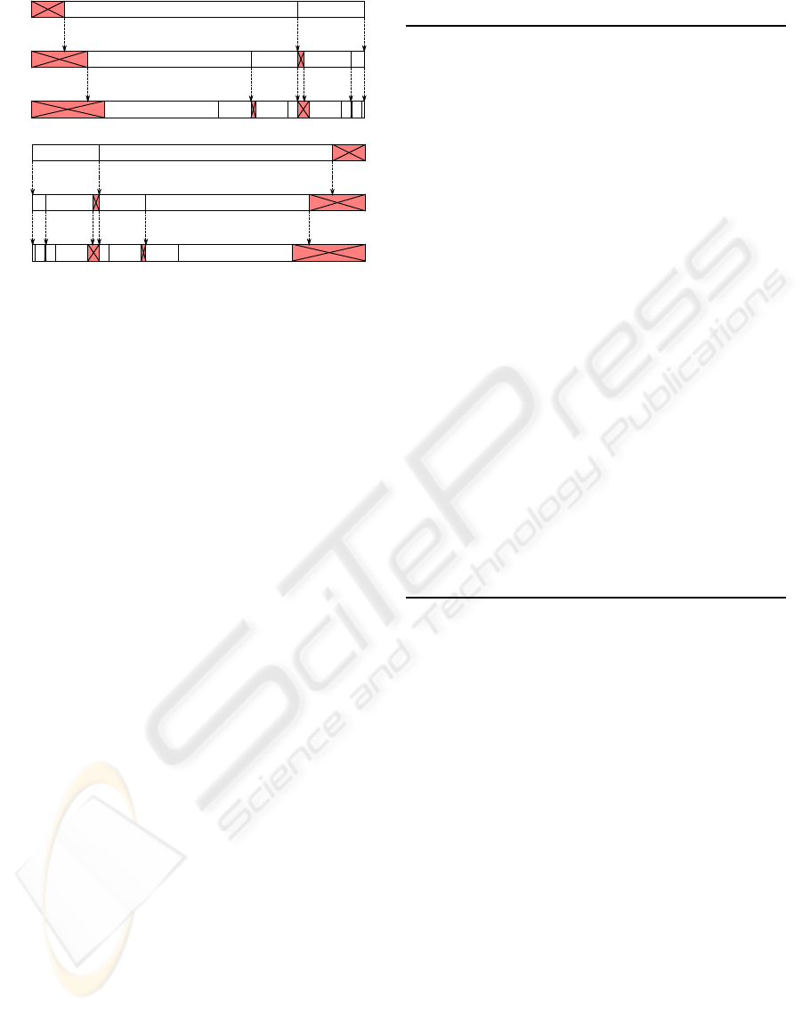
(a)

a b

bbbaabaa

aaa aab aba baa

(b)

abaa bbba

bba bbbabb bab

Figure 3: Forbidden gaps after three stages when placed

to reduce error-detection delay for (a) P(a) > P(b) and (b)

P(a) < P(b).

bols as shown in Figure 3 (a). If P(a) < P(b), the

forbidden gap should be placed after the symbols as

shown in Figure 3 (b). If P(a) = P(b), no advantage

is observed by changing the forbidden gap placement.

Ben-Jamaa, Weidmann and Kieffer (2008) split

the forbidden gap into three parts for binary-source

arithmetic codes, one part before the ﬁrst symbol sub-

interval, the second between the two sub-intervals,

and the third after the second sub-interval. Their

results show that the worst performance is obtained

when the gap is completely between the two sub-

intervals.

When the model is adaptive, it may be that some-

times P(a) > P(b) and sometimes P(a) < P(b). This

placement scheme needs some modiﬁcation to work

with such a model. When encoding a symbol, the

ﬁrst thing to do is to ﬁnd the most probable symbol.

The sub-interval for this symbol is then swapped with

the ﬁrst sub-interval. Then, the forbidden gap can be

placed at the beginning of the interval.

Section 4.1 presents experimental results for plac-

ing the forbidden gap at the beginning, at the middle,

and at the end of the interval.

3.2 Looking Ahead during Decoding

During regular decoding of arithmetic codes (Witten

et al., 1987), two interval values are maintained, one

is the decodinginterval, which is the same as the inter-

val produced by the encoder, and the other is the input

codeword interval, which depends directly on the bit

sequence being decoded. For a symbol to be decoded,

the input interval has to lie completely within one of

the sub-intervals of the decoding interval. The for-

bidden gap technique detects an error when the input

interval lies completely within a forbidden gap.

When decoding arithmetic codes with a forbidden

Table 1: Look-ahead decoding steps for each bit.

1: Initially, the input interval is [l

, h

the decoding interval is split into S sub-intervals

, h

), [l

, h

), ···, [l

, h

), and

is the assumed transmitted bit.

2: if t

= 0 then

3: h

⇐ (l

+ h

)/2

4: else

5: l

⇐ (l

+ h

)/2

6: end if

7: Search for symbols s with their corresponding

sub-interval [l

, h

) overlapping the input interval

, h

), that is, l

< h

and h

> l

8: if no matching symbols are found then

9: Flag an error.

10: else if only one matching symbol is found then

11: Add found symbol s to the list of decoded sym-

bols.

12: Scale the region [l

, h

) if necessary, scaling [l

) in the same way.

13: Split the scaled [l

, h

) into S new sub-intervals

′

, h

′

), [l

′

, h

′

), ···, [l

′

, h

′

14: l

⇐ l

′

, h

⇐ h

′

, l

⇐ l

′

, h

⇐ h

′

, ··· , l

⇐

′

, h

⇐ h

′

15: Go to 7.

16: else {more than one matching symbol is found}

17: Go to 19.

18: end if

19: End.

gap, sometimes we can decode a symbol even though

the input interval is not completely within the sub-

interval corresponding to the symbol. If the input

interval is divided between one sub-interval and the

forbidden gap, there is only one symbol that can be

decoded, the symbol corresponding to that one sub-

interval. In this case, we can decode the symbol im-

mediately and for the moment assume that the bit se-

quence is not in error. We still need to keep track of

the input interval. When we look ahead in this way,

we may be able to detect errors earlier. Table 1 shows

how the look-ahead decoder handles an input bit.

When using look-ahead, the input interval does

not need to lie completely within the decoding inter-

val. But since the symbol is decoded, the decoding

interval and the input codeword interval have to be

normalized, that is, the intervals have to be doubled

in size. Since the input interval can be larger than the

decoding interval, it is possible for the input interval,

denoted by [l

, h

) in Table 1, to extend out of the [0, 1)

interval. So in the implementation, it is important to

cater for the possibility that l

< 0 or that h

≥ 1.

Section 4.1 presents experimental results indicat-

ing how much the look-ahead technique advances the

detection of errors, while Section 4.2 shows the gain

SIGMAP 2010 - International Conference on Signal Processing and Multimedia Applications

obtained when using this technique in MAP decoding

of arithmetic codes.

3.3 Updating the Prior Probability

Continuously

In Section 2.2.1, both the metric for hard-decision de-

coding shown in (14) and the metric for soft-decision

decoding shown in (19) have a component for the

prior probability P(u). Recall that this component,

logP(u

), is calculated using

logP(u

) =

∑

i=1

logP(u

n,i

), (11)

where I ≥ 0 is the number of symbols that can be de-

coded assuming the transmitted bit t

There is another way to calculate the prior proba-

bility. In arithmetic coding, the width of the interval

is directly related to the probability of the source sym-

bols. Ignoring the forbidden gaps for the moment, we

can say that for an input sequence u

, u

, ··· , u

Interval width = P(u) =

∏

l=1

P(u

). (20)

In arithmetic coding algorithms, whenever a bit is

emitted by the encoder, the message interval is scaled

by a factor of 2 (Witten et al., 1987). This normaliza-

tion process always leaves the message interval with a

width in the range (0.25,1]. If to encode the input se-

quence u the encoder emits N bits, the interval width

is scaled by a total factor of 2

. Also, the ﬁnal scaled

width of the interval is in the range (0.25, 1], that is,

it is approximately 1. If we ignore termination, which

at most uses two bits (Witten et al., 1987),

P(u) = 1 (21)

P(u) = 2

−N

(22)

logP(u) = −N log2 (23)

logP(u

) = −log2. (24)

All we have to do to the additive MAP metric to cater

for the prior probability is to subtract log2 for each

decoded bit.

In the above, we have ignored the effect of forbid-

den gaps on the interval width. Compensating for for-

bidden gaps is not very difﬁcult. Every time there is a

forbidden gap, that is, for each symbol encoded or de-

coded, the interval is reduced by a factor of (1−ε). To

compensate for this, for each decoded symbol we sub-

tract log(1−ε) from the metric. Note that (1−ε) < 1,

so we are subtracting a negative number, and the met-

ric is increasing, not decreasing.

Section 4.2 presents experimental results show-

ing the gain obtained when using this improvement

in MAP decoding of arithmetic codes.

4 RESULTS

4.1 Placing the Forbidden Gap

Experiments were performed to test the forbidden gap

placement mentioned in Section 3.1. The test was per-

formed for a binary source model with alphabet con-

taining symbols a and b in the following scenarios:

1. Fixed model, forbidden gap placed at the begin-

ning of the interval.

2. Fixed model, forbidden gap placed at the begin-

ning of the interval, look-ahead.

3. Fixed model, forbidden gap placed in the middle

of the interval.

4. Fixed model, forbidden gap placed in the middle

of the interval, look-ahead.

5. Fixed model, forbidden gap placed at the end of

the interval.

6. Fixed model, forbidden gap placed at the end of

the interval, look-ahead.

7. Adaptive model, forbidden gap placed at the be-

ginning of the interval.

8. Adaptive model, forbidden gap placed at the be-

ginning of the interval, look-ahead.

9. Adaptive model, forbidden gap placed in the mid-

dle of the interval.

10. Adaptive model, forbidden gap placed in the mid-

dle of the interval, look-ahead

11. Adaptive model, forbidden gap placed in the be-

ginning of the interval, with the sub-interval for

the most probable symbol moved towards the be-

ginning of the interval.

12. Adaptive model, forbidden gap placed in the be-

ginning of the interval, with the sub-interval for

the most probable symbol moved towards the be-

ginning of the interval, look-ahead.

The error-detection delay was measured for different

values of P(a), where P(a) is the probability of the

ﬁrst symbol. Each test was performed using no look-

ahead and using look-ahead mentioned in Section 3.2.

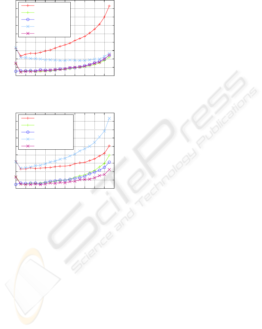
Figure 4 shows the results for a static source

model with a code rate of 8/9 (scenarios 1–6). With-

out look-ahead, placing the forbidden gap at the be-

ginning of the interval suffers the largest delay, but

with look-ahead, placing the forbidden gap at the be-

ginning of the interval achieves the smallest delay.

When the probability of the ﬁrst symbol in the

interval is larger than the probability of the second

ARITHMETIC CODING FOR JOINT SOURCE-CHANNEL CODING

0.5 0.55 0.6 0.65 0.7 0.75 0.8 0.85 0.9 0.95 1

Delay (bits)

P(a)

Scenario 1

Scenario 2

Scenario 3/4

Scenario 5

Scenario 6

Figure 4: Error-detection delay for static source model with

a code rate of 8/9.

0.5 0.55 0.6 0.65 0.7 0.75 0.8 0.85 0.9 0.95 1

Delay (bits)

P(a)

Scenario 7

Scenario 8

Scenario 9/10

Scenario 11

Scenario 12

Figure 5: Error-detection delay for adaptive source model

with a code rate of 8/9.

symbol, and the forbidden gap is placed at the begin-

ning of the interval, forbidden gaps tend to cluster to-

gether, as shown in Figure 3 (a). Without look-ahead,

this seems to make the delay larger. This may be be-

cause concentrating the gaps at fewer places makes

it harder for a random interval (a bit error makes the

interval seem random) to ﬁnd one of the gaps and lie

completely within it. With look-ahead, the situation

is reversed, now having the gaps clustered makes the

look-ahead technique more effective.

Figure 5 shows the results for an adaptive source

model with a code rate of 8/9 (scenarios 7–11). The

performance of scenarios 11 and 12 is similar to the

performance of scenarios 1 and 2. Without look-

ahead, this scheme suffers the largest delay, and with

look-ahead, it achieves the smallest delay.

The results for scenarios 3 and 4 are identical.

This shows that look-ahead does not help when the

forbidden gap is in the middle of the interval. This

may be because with this scheme, forbidden gaps are

never next to each other. In the graphs, only one of

these scenarios is plotted. The same can be said for

scenarios 9 and 10.

Both Figures 4 and 5 show an increase in the de-

tection delay at P(a) = 0.5. This effect is worth ex-

plaining. Since the probability of both symbols is

P(a) = P(b) = 0.5, exactly 1 bit is needed to encode

each symbol. Also, for a code rate of 8/9, an ex-

tra 1/8 of a bit is used for each forbidden gap. As-

suming no rounding errors, after 8 gaps have been in-

serted, the total number of bits used by the gaps is

1 and has no fractional part. Thus, an exact number

of bits have been used, so for the next symbol, the

boundaries of the sub-intervals for a and b will lie on

the bit boundaries, with the consequence that a bit er-

ror will cleanly switch the encoded symbol and will

not be detectable. This occurs for every 8 encoded

symbols, which means that for the given probabilities

and code rate, one every nine bits is susceptible to an

undetectable error. Because of rounding errors, the

number of bits for each forbidden gap will not be ex-

actly 1/8, so the number of bits used for 8 gaps will

havea tiny fractional part, and errors in these sensitive

bits will be detectable, but the sub-intervalboundaries

for the sensitive symbols are still very close to the bit

boundaries, resulting in a longer detection delay and

a higher average delay for P(a) = 0.5. This has been

veriﬁed experimentally. When the gap is placed in

the middle (scenarios 3/4 and 9/10), the sub-interval

boundaries cannot be on bit boundaries for both sym-

bols, so the effect does not happen. In practice this

effect is not really worrisome; if P(a) = P(b) = 0.5

throughout the message, the message is not compress-

ible, so arithmetic coding is not used.

4.2 MAP Decoding

Simulations were preformed to test the MAP decod-

ing algorithms. The source used was similar to that

used in Grangetto et al. (2005), to make the compari-

son fair.

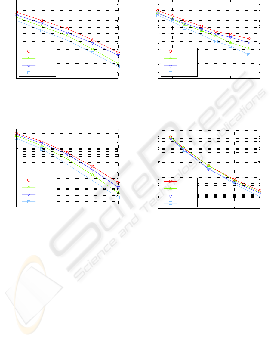
Figure 6 shows the packet error rate (PER) for

a static binary source model using hard-decision de-

coding. The stack size M = 256, and the gap factor

ε = 0.185. Figure 7 shows the PER for the same con-

ditions using soft-decision decoding.

The performance is improved when the look-

ahead technique of Section 3.2 is used. When this

technique is used, the decoder may detect errors ear-

lier, and it can detect correct symbols earlier as well.

When errors are detected early, incorrect paths can be

pruned earlier from the decoding tree, reducing the

chance that the correct path is removed because of a

stack overﬂow. Detecting symbols early will enable

the MAP metric to be updated earlier, which can lead

SIGMAP 2010 - International Conference on Signal Processing and Multimedia Applications

-4

-3

-2

-1

4 4.5 5 5.5 6

PER

(dB)

NLA PS

LA PS

NLA PB

LA PB

Figure 6: Performance for MAP hard-decision decoder for

static binary model with M = 256 and ε = 0.185; without

look-ahead (NLA) and with look-ahead (LA); and with P(t)

adjusted every symbol (PS) or every bit (PB).

-4

-3

-2

-1

1 1.5 2 2.5 3

PER

(dB)

NLA PS

LA PS

NLA PB

LA PB

Figure 7: Performance for MAP soft-decision decoder for

static binary model with M = 256 and ε = 0.185; without

look-ahead (NLA) and with look-ahead (LA); and with P(t)

adjusted every symbol (PS) or every bit (PB).

to better decoding. The performance is also improved

with continuous updating of the prior probability P(t)

as described in Section 3.3, that is, when P(t) is ad-

justed every time we decode a bit rather than every

time we decode a symbol. The performance is im-

proved most when the techniques are used together.

Figures 8 and 9 show how the PER changes with

ε when E

is ﬁxed at 5.5 dB for hard-decision de-

coding and soft-decision decoding respectively. The

improved schemes can achieve the error-correction

performance of the original scheme using less redun-

dancy. For example, for a PER of 10

−2

, the hard-

decision decoder for the original scheme needs ε =

0.19, which translates into a code rate of 0.65. For

the same PER, the hard-decision decoder for the im-

proved scheme needs ε = 0.13, which translates into

a code rate of 0.73.

-4

-3

-2

-1

0.06 0.08 0.1 0.12 0.14 0.16 0.18 0.2

PER

NLA PS

LA PS

NLA PB

LA PB

Figure 8: Performance for MAP hard-decision decoder for

static binary model with M = 256 and E

= 5.5 dB;

without look-ahead (NLA) and with look-ahead (LA); and

with P(t) adjusted every symbol (PS) or every bit (PB).

-5

-4

-3

-2

-1

0 0.01 0.02 0.03 0.04

PER

NLA PS

LA PS

NLA PB

LA PB

Figure 9: Performance for MAP soft-decision decoder for

static binary model with M = 256 and E

= 5.5 dB;

without look-ahead (NLA) and with look-ahead (LA); and

with P(t) adjusted every symbol (PS) or every bit (PB).

In all graphs, the plot for the scheme with no im-

provements, that is with no look-ahead and with the

prior probability P(t) updated after every symbol in-

stead of after every bit, is comparable to the plots pub-

lished by Grangetto et al. (2005).

5 CONCLUSIONS

In this paper, a joint source-channel arithmetic MAP

decoder proposed by Grangetto et al. (2005) for de-

coding arithmetic codes with a forbidden symbol

transmitted over an AWGN channel was analysed.

Novel techniques were introduced to improve the

error-correction performance of the code. The arith-

metic decoder was improved with a look-ahead tech-

ARITHMETIC CODING FOR JOINT SOURCE-CHANNEL CODING

nique that enables it to detect errors earlier. When

using the MAP decoder, this improves the PER at the

cost of a small increase in complexity. The MAP met-

ric calculation was changed by improving the way the

prior probability component of the metric is updated,

leading to faster updating of the metric and, conse-

quently, to a better error-correctionperformance. This

technique makes the MAP decoder faster as well be-

cause the better path in the MAP tree is found ear-

lier. A coding gain of up to 0.4 dB for soft-decision

decoding and 0.6 dB for hard-decision decoding was

observed for a code rate of 2/3 and M = 256. A num-

ber of multimedia applications are using arithmetic

coding as the ﬁnal entropy coding stage, making a

joint-source channel coding scheme based on arith-

metic coding attractive for wireless multimedia trans-

mission.

REFERENCES

Bahl, L. R., Cocke, J., Jelinek, F., and Raviv, J. (1974). Op-

timal decoding of linear codes for minimizing symbol

error rate. IEEE Transactions on Information Theory,

20(2):284–287.

Ben-Jamaa, S., Weidmann, C., and Kieffer, M. (2008). An-

alytical tools for optimizing the error correction per-

formance of arithmetic codes. IEEE Transactions on

Communications, 56(9):1458–1468.

Bi, D., Hoffman, M. W., and Sayood, K. (2010). Joint

Source Channel Coding Using Arithmetic Codes.

Synthesis Lectures on Communications. Morgan &

Claypool Publishers.

Boyd, C., Cleary, J. G., Irvine, S. A., Rinsma-Melchert, I.,

and Witten, I. H. (1997). Integrating error detection

into arithmetic coding. IEEE Transactions on Com-

munications, 45(1):1–3.

Grangetto, M., Cosman, P., and Olmo, G. (2005). Joint

source/channel coding and MAP decoding of arith-

metic codes. IEEE Transactions on Communications,

53(6):1007–1016.

Grangetto, M., Scanavino, B., Olmo, G., and Benedetto,

S. (2007). Iterative decoding of serially concatenated

arithmetic and channel codes with jpeg 2000 appli-

cations. IEEE Transactions on Image Processing,

16(6):1557–1567.

Guionnet, T. and Guillemot, C. (2003). Soft decoding and

synchronization of arithmetic codes: Application to

image transmission over noisy channels. IEEE Trans-

actions on Image Processing, 12(12):1599–1609.

Hagenauer, J. (1988). Rate-compatible punctured convo-

lutional codes (RCPC codes) and their applications.

IEEE Transactions on Communications, 36(4):389–

400.

Huffman, D. A. (1952). A method for the construction of

minimum-redundancy codes. Proceedings of the IRE,

40(9):1098–1101.

Jelinek, F. (1969). Fast sequential decoding algorithm using

a stack. IBM Journal of Research and Development,

13(6):675–685.

Lelewer, D. A. and Hirschberg, D. S. (1987). Data com-

pression. ACM Computing Surveys, 3:261–296.

MacKay, D. J. C. (2003). Information Theory, Inference,

and Learning Algorithms, chapter 25, pages 324–333.

Cambridge University Press.

Park, M. and Miller, D. J. (2000). Joint source-channel de-

coding for variable-length encoded data by exact and

approximate MAP sequence estimation. IEEE Trans-

actions on Communications, 48(1):1–6.

Rissanen, J. J. (1976). Generalized Kraft inequality and

arithmetic coding. IBM Journal of Research and De-

velopment, 20(3):198–203.

Sayir, J. (1999). Arithmetic coding for noisy channels.

In Proceedings of the 1999 IEEE Information Theory

and Communications Workshop, pages 69–71.

Shannon, C. E. (1948). A mathematical theory of commu-

nication. Bell System Technical Journal, 27:379–423.

Vembu, S., Verd`u, S., and Steinberg, Y. (1995). The source-

channel separation theorem revisited. IEEE Transac-

tions on Information Theory, 41(1):44–54.

Witten, I. H., Neal, R. M., and Cleary, J. G. (1987). Arith-

metic coding for data compression. Communications

of the ACM, 30(6):520–540.

SIGMAP 2010 - International Conference on Signal Processing and Multimedia Applications