
DESIGN OF A MULTIOBJECTIVE PREDICTIVE CONTROLLER
FOR MULTIVARIABLE SYSTEMS
F. Ben Aicha, F. Bouani and M. Ksouri
Laboratory of Analysis and Control of Systems, National Engineering School of Tunis
BP 37, le Belvedere 1002, Tunis, Tunisia
Keywords: Generalized predictive control, Multiobjective optimization, Multivariable systems, Decentralized control,
Decouplers, Genetic algorithm.
Abstract: In this paper, a strategy for automatic tuning of decentralized predictive controller synthesis parameters
based on multiobjective optimization for multivariable systems is proposed. This strategy integrates the
genetic algorithm to generate the synthesis parameters (the prediction horizon, the control horizon and the
cost weighting factor) making a compromise between closed loop performances (the overshoot, the variance
of the control and the settling time). A simulation example is presented to illustrate the performance of this
strategy in the on-line adjustment of generalized predictive control parameters.
1 INTRODUCTION
Processes with only one output being controlled by a
single manipulated variable are classified as single-
input single output (SISO) systems. Many processes,
however, do not conform to such simple control
configuration. These systems are known as multi-
input multi-output (MIMO) or multivariable
systems. As most of the multivariable systems
present interactions, the interaction problem between
control loops has long been recognised as an area for
concern and many approaches to deal with this
problem were proposed. The method used in this
work is to design non-interacting or decoupling
controllers to eliminate completely the effects of
loop interactions. This is achieved via decouplers
(Albertos and Sala, 2004). As a control technique,
we have used the Generalized Predictive Control
(GPC) which has achieved great success in practical
applications in recent decades. This strategy of
control requires the determination of synthesis
parameters: prediction horizon, control horizon and
cost weighting factor which give acceptable closed
loop performances. But, there is not exact rules
giving the values of required parameters. Some
works deal with the automatic tuning of GPC such
as (Ben Abdennour, Ksouri and Favier, 1998) in
which, an on-line adjustment of GPC’s synthesis
parameters using the fuzzy logic is presented. But,
this method does not give exact values of synthesis
parameters but allows a fuzzy description of each
parameter (small, average, big). On the other hand,
in (Ben Abdennour, Ksouri and Favier, 1998) to
determine the GPC parameters, each performance
criterion is minimized without considering the others
criteria, so the problem is considered as a single-
objective one. In practice, the optimization problems
are rarely single-objective; where from the interest
of multiobjective optimization (MOO) based on the
minimization of all performance criteria at every
sample time. The MOO leads to a set of optimal
solutions, i.e. the Pareto optimal solutions or the non
dominated solutions (Collette and Siarry, 2002). In
this context, many works such as (Popov, Farag and
Werner, 2005), (Yang and Pedersen, 2006),
(Bemporada and Muñoz de la Peñab, 2009) and
(Muldera, Tiwari and Kothare, 2009) were interested
in the synthesis of controllers based on
multiobjective optimisation which has more and
more interest. In this paper, we propose a new
method allowing the on-line adjustment of synthesis
parameters of predictive controller using the genetic
algorithm and that for the multivariable systems.
The performances’ criteria to be simultaneously
minimized are the settling time, the overshoot and
the variance of the control. This paper is organized
as follows. The problem is formulated in section two
where the multivariable decoupling control and the
predictive control principle are given. The proposed
109
Ben Aicha F., Bouani F. and Ksouri M. (2010).
DESIGN OF A MULTIOBJECTIVE PREDICTIVE CONTROLLER FOR MULTIVARIABLE SYSTEMS.
In Proceedings of the 7th International Conference on Informatics in Control, Automation and Robotics, pages 109-115
DOI: 10.5220/0002945001090115
Copyright
c
SciTePress

method allowing the tuning of synthesis parameters
and the design of the multiobjective predictive
controller are described in section three. The
obtained simulation results are presented in section
four. Conclusions are given in the last section.
2 PROBLEM FORMULATION
2.1 Multivariable System
Representation
We consider a multivariable linear system with m
inputs u
i
(k): i=1,…,m and n outputs y
j
(k) : j=1,…,n.
The system equation is given by:
1
() ( ) ()Yk Gz Uk
−
=
(1)
with:
12
( ) [ ( ), ( ),...., ( )]
T
m
Uk u k u k u k= is the control
vector,
12
() [ (), (),....., ()]
T
n
Yk y k y k y k= is the output
vector and
()
1
Gz
−
is the transfer function matrix
having as dimension mn× given by:
11
11 1
1
11
1
() ()
()
() ()
m
nnm
gz g z
Gz
gz g z
−−
−
−−
⎛⎞
⎜⎟
=
⎜⎟
⎜⎟
⎝⎠
"
#% #
"
(2)
For the P canonical structure (Albertos and Sala,
2004)., in the case of a system with two inputs and
two outputs, the outputs are related to the inputs
according to:
11
1111122
() ()() ()()
y
k gzuk gzuk
−−
=+
(3)
11
2222211
() ( ) () ( ) ()
y
k gzuk gzuk
−−
=+
(4)
2.2 Multivariable Decoupling Control
Generally, in the industry the distributed control is
the most favorable and the most used thanks to its
structure simplicity. During the decentralized control
design for a two inputs two outputs (TITO) process,
the input-output pairing is essential and determining
for the obtained performances as well as for the
stability of the system (Moaveni and Khaki-Sedigh,
2006). Several methods were proposed to solve the
interaction problem (Bristol, 1966), (Khelassi,
Wilson and Bendib, 2004). The method which will
be applied in this work is the one using decouplers
having as role to decompose a multivariable process
into a series of independent single-loop sub-systems,
and the multivariable process can be controlled
using independent loop controllers. As well as the
input-output representation of multivariable
processes, different structures are possible, like P or
V decouplers. Judging by the literature, the P-
decoupler seems to be the most popular. In this
work, we choose to use the decoupling network of
Zalkind given in (Zalkind, 1967). The structure of
the obtained decoupled process having as auxilliary
inputs
1
()vk and
2
()vk is presented in the figure
below.
Figure 1: The structure of the decoupled process.
The control signals are given by:
11
1111122
() ( ) () ( ) ()uk D z vk D z vk
−−
=+
(5)
11
2211222
() ( ) () ( ) ()uk D z vk D z vk
−−
=+
(6)
where
-1
(), 1,2 1,2
ij
D z i and j== are the elements
of the transfer function
-1
()Dz .
In taking into account equations (3), (4), (5) and (6),
we shall have:
11 11
1 1111 2112 1
11 11
22 12 12 11 2
() ()() ()()()
( ) ( ) ( ) ( ) ( )
yk D z g z D z g z vk
Dzgz Dzgz vk
−− −−
−− −−
⎡⎤
=+
⎢⎥
⎣⎦
⎡⎤
++
⎢⎥
⎣⎦
(7)
11 11
2 1121 2122 1
11 11
22 22 12 21 2
() ()() ()()()
()() ()()()
y
k Dzgz Dzgz vk
Dzgz Dzgz vk
−− −−
−− −−
⎡⎤
=+
⎢⎥
⎣⎦
⎡⎤
++
⎢⎥
⎣⎦
(8)
To have y
2
(k) independent of v
1
(k) and y
1
(k)
independent of v
2
(k), we introduce the decouplers
between the process and the controller such as :
12 22
12
11
() ()
()
()
g
zD z
Dz
gz
−
=
(9)
21 11
21
22
() ()
()
()
g
zD z
Dz
gz
−
=
(10)
Generally we take D
11
(z)=1 and D
22
(z)=1 except in
case the delays are more important in the direct
branches than in the crossed branches (Albertos and
Sala, 2004).
By using (9) and (10) in (7) and (8), we obtain:
-1 -1
-1
12 21
111 1
-1
22
() ()
() ( )- ()
()
gzgz
yk g z vk
gz
⎛⎞
=
⎜⎟
⎜⎟
⎝⎠
(11)
1
()Gz
−
1
()
D
z
−
y
1
(k)
y
2
(k)
u
1
(k)
u
2
(k)
v
1
(k)
v
2
(k)
ICINCO 2010 - 7th International Conference on Informatics in Control, Automation and Robotics
110

-1 -1
-1
12 21
222 2
-1
11
() ()
() ( )- ()
()
gzgz
yk g z vk
gz
⎛⎞
=
⎜⎟
⎜⎟
⎝⎠
(12)
The use of (9) and (10) leads to the following
control signals:
-
-
()
() () ()
()
1
12
121
1
11
gz
uk vk vk
gz
−
=+
(13)
-
-
()
() () ()
()
1
21
212
1
22
gz
uk vk vk
gz
−
=+
(14)
The (
mn×
) multivariable process is treated as a set
of n SISO processes. Each SISO process is
characterized by a CARIMA (Controlled Auto
Regressive Integrated Moving Average) dynamic
model. This model is given by the following
relation:
()
() () () v( ) ()
()
1
1d1
1
Cz
A
zykzBz k1 ek
z
−
−−−
−
=−+
Δ
(15)
where
-
()yk and ()vk are respectively the output and the
input of the system.
-
()ek is a sequence of white noise with zero mean
average and a finite variance.
-The polynomials
()
1
A
z
−
, ()
1
B
z
−
, ()
1
Cz
−
and ()
1
z
−
Δ
are given by:
( ) .....
11 nA
1nA
Az 1 az a z
−− −
=+ + +
(16)
( ) .....
11 nB
01 nB
Bz b bz b z
−− −
=+ + +
(17)
( ) .....
11 nC
1nC
Cz 1 cz c z
−− −
=+ + +
(18)
()
11
z1z
−−
Δ=−
(19)
-The roots in z of
()
1
Cz
−
must be strictly inside the
unit circle.
- d represents the time delay of the system.
2.3 The GPC Optimal Control
The generalized predictive control is based on the
minimization of a quadratic criterion given by the
following expression (Richalet, Lavielle and Mallet,
2005), (Clarke, Mohtadi and Tuffs, 1987):
ˆ
( ( )- ( / )) ( ( ))
Hp d
Hc 1
j1d j0
GPC
22
J
c
rk j yk jk vk j
+
−
=+ =
= +++ρΔ+
∑∑
(20)
where
p
H
is the prediction horizon,
c
H
is the control
horizon,
ρ
is the cost weighting factor, ()
c
rk is the
set point,
ˆ
(/)
y
kjk
+
is the predicted output
and
()kjv
+
Δ
is the future increments of the control
given by:
()()( 1)vk j vk j vk j
Δ
+= +− +−
(21)
By minimizing the criterion
GPC
J , we can determine
the expression of the optimal vector
() (),..., ( 1)
T
c
Vk vk vk HΔ=Δ Δ+−
⎡
⎤
⎣
⎦
as follows:
() () [ () ( )( )]
()
1
1
1
Vk K R k Gyk R z vk 1
GPC c
Cz
−
−
Δ= − +Δ −
⎡
⎤
⎡
⎤
⎢
⎥
⎢
⎥
⎢
⎥
⎢
⎥
⎣
⎦
⎣
⎦
(21)
where
GPC
K =[]
c
T1T
11 1
H
INN N
−
+ρ
(23)
( ) [ ( ),..., ( )] .
T
cc c
p
krk1drkHdR =++ ++
(24)
1
N is a
(,)
pc
H
H
matrix, G and R are obtained by
the resolution of Diophantine equations (Clarke,
Mohtadi, and Tuffs, 1987). The optimal control to be
applied to the process is defined from the vector
given by (22) using the receding horizon principle.
This optimal control
()vk is computed from the first
element
()v1
Δ
of the vector ()VkΔ :
() ( 1) (1)vk vk v
=
−+Δ
(25)
It is evident that the optimal predictive control
depends on synthesis parameters
(, , )
pc
HHρ
. So, in
this paper, we present a new method allowing the
automatic determination of required GPC’s synthesis
parameters in the case of multivariable systems.
3 MULTIOBJECTIVE
GENERALIZED PREDICTIVE
CONTROL
Multi-objective optimization (MOO) can be defined
as the problem of finding a vector of
parameters
[
]
,...,
T
1l
X
xx=
, which optimizes a
vector of objective functions
( ,..., )
1n
J
J (Gambier,
2008). In general, the MOO problem can be
formulated as follows:
min ((), (),..., ())
12 n
X
JXJX JX
(26)
DESIGN OF A MULTIOBJECTIVE PREDICTIVE CONTROLLER FOR MULTIVARIABLE SYSTEMS
111
At present, a very huge number of methods to solve
MOO problems can be found in literature (Collette
and Siarry, 2002), (Gambier, 2008). The method
applied in this work is the weighted sum method that
belongs to the family of aggregative methods.
3.1 Weighted Sum Method
This method allows the transformation of the
objective functions vector in a single-objective
function. It is known for its efficiency and suitability
to generate a strongly non dominated solution that
can be used as an initial solution for other
techniques. The single criterion is obtained by the
sum of the weighted criteria as follows (Gambier,
2008):
n
ii
i1
J
wJ
=
=
∑
(27)
where the weights are chosen such that:
=
n
ii
i1
w1and0w1
=
≤≤
∑
(28)
The MOO leads to a set of solutions known as a
Pareto set. This set is also called non-dominated
solutions. When the non dominated solutions are
collectively plotted in the criterion space, they
constitute the Pareto front (Gambier, 2008). All
points of the Pareto front are equally acceptable
solution for the problem. However, it is necessary to
obtain only one point in order to be able to
implement the controller (Gambier, 2008).To choose
one solution from the Pareto front, we can compute
the following norm for each solution which gives a
compromise between all criteria (Bouani, Laabidi,
and Ksouri, 2006):
22 2
12
...
in
dJJ J =+++
(29)
The quality of a control applied to a process is
generally estimated by the closed loop performances
of the system. Among these performances we
choose as objective functions to optimize:
The overshoot
%
D
max
%
c
c
y
r
D 100
r
−
=
(30)
max
y is the maximum value of the output and
c
r is
the set point value.
The variance of the control
v
V
()
2
1
N
2
N
v
21
vk
V
NN
∑
=
−
(31)
1
N is the first measure iteration and
2
N is the last
one.
The settling time
s
T : It is the first instant after
which, the system output doesn’t exceed
%5± of
the set point value.
So, to estimate the synthesis parameters for GPC,
the following criterion will be minimized.
%
.
12v3s
J
wD wV wT
=
++
(32)
such that:
123
www1
+
+=and ; ,...,
i
0w1 i1 3
≤
≤= .
3.2 Generating Optimal Solutions
Using Genetic Algorithms
In genetic algorithms, each parameter is represented
by a string structure. This is similar to the
chromosome structure in natural genes (Goldberg,
1991). A group of strings are called population. It
should be notice that GAs evaluate a set of solutions
in the population at each iteration step. Every
solution is formed by GPC’s synthesis parameters. A
number of genetic operators (selection, crossover
and mutation) are available to generate new
individuals in next generation.
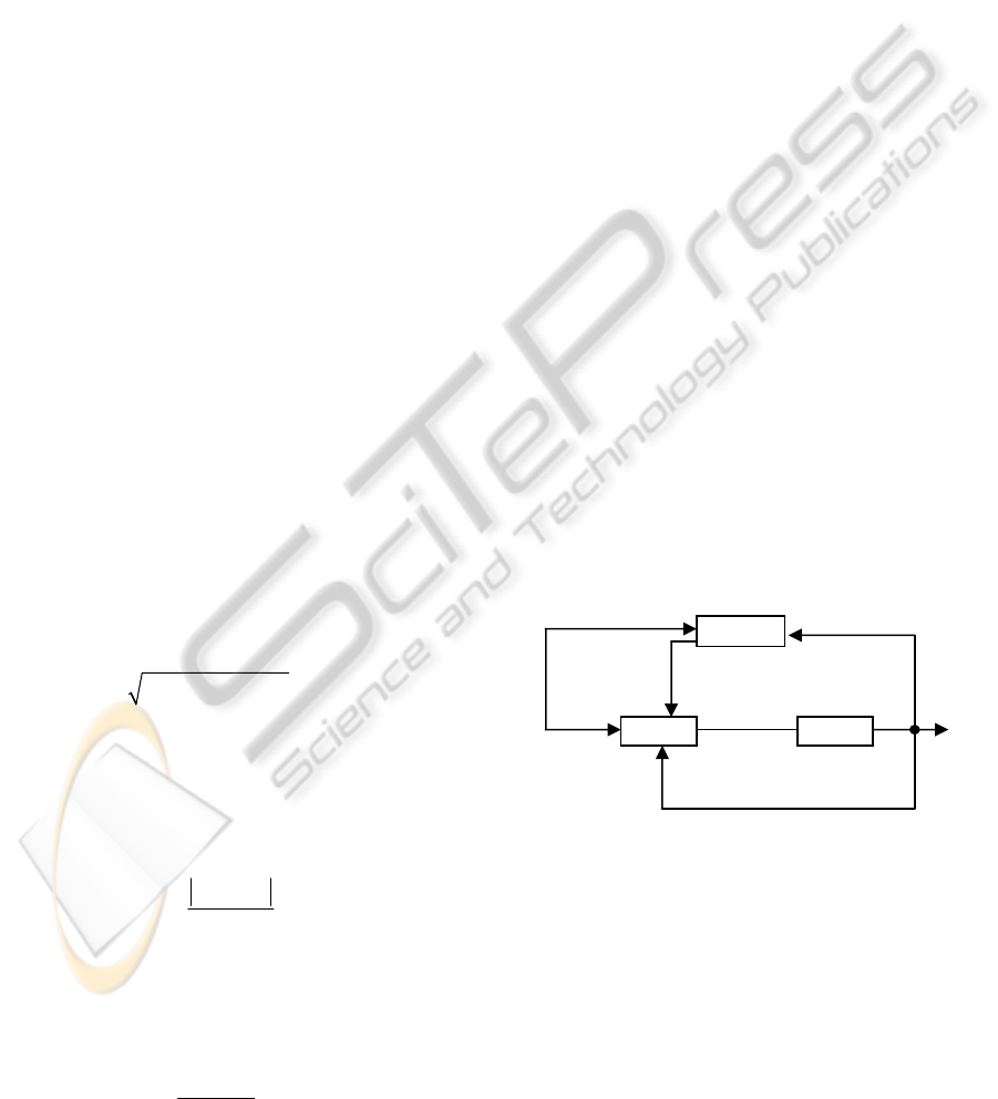
In this paper, we propose an on-line supervisor for
each classic predictive controller based on genetic
algorithms. In figure 2, we present the structure of
this supervisor. Each supervisor permits the on-line
adjustment of the GPC algorithm parameters in
order to optimize simultaneously closed loop
performances.
Figure 2: The Supervisor of the Classic Predictive
Controller.
In our work, the GA population is formed by the
synthesis parameters (
p
H
,
c
H
,ρ ). The initial
population is formed by arbitrary values, such as:
p
1H 20
≤
≤
;
c
1H 3
≤
≤ and
010<ρ≤
. For each
individual of the population, we use the process
model and the generalized predictive controller in
order to compute, for a given set point, the output
sequence along two hundreds sample times. Then,
we evaluate the performance indices (
%
D ,
v
V ,
s
T )
Supervisor
Process GPC
()yk
()uk
,,
pc
HH
ρ
(),...,( )
ccp
rk rk H
+
ICINCO 2010 - 7th International Conference on Informatics in Control, Automation and Robotics
112

and the fitness. To obtain the new population, we
use the roulette wheel as a selection operator. To
acquire more information in the new population, the
crossover and the mutation operators are needed.
This procedure will be repeated until a stop criterion
(e.g. max number of generation) is reached. Then,
we obtain the best individual (optimal values of
p
H
,
c
H
andρ ) that minimizes the performances
indices. The steps used to compute the best synthesis
parameters are given in algorithm 1. In this
algorithm, we design by max_gen the maximum
number of generations and by max_pop the
maximum number of population.
Algorithm 1: The principal steps to design multi-objective
predictive controller.
Form the initial population
For j=1 To max_gen
For i=1 To max_pop
-
Take the ith individual of the population,
-
Use the GPC with the process model,
-
Compute the model output,
-
Evaluate the criteria:
%
D ,
v
V ,
s
T
-
Evaluate the fitness using (32)
End
Use the GA operators (selection, crossover and
mutation) to form the new population.
End
Take the best individual
(,,)
pc
HHρ
.
Once the non dominated solutions are computed, the
problem is which solution can be used with the GPC
to handle the real process. To choose one solution
from the Pareto front, we compute the following
norm for each solution:
222
%
.
ivs
dDVT =++
(33)
The steps allowing to find the synthesis parameters
which minimize the performance criteria, given by
the proposed algorithm is executed twice because
the TITO system is decomposed into two
monovariable systems controlled each by
multiobjective predictive controller.
4 SIMULATION RESULTS
To estimate the closed loop performances obtained
by applying the approach presented in this paper, we
consider the TITO process given in (Miskovic,
Karimi, Bonvin and Gevers, 2007) characterized by
the next transfer functions matrix:
. z . z
. z . z
()
. z . z
. z . z
11
11
1
11
11
0 09516 0 03807
1 0 9048 1 0 9048
Gz
0 02974 0 04758
1 0 9048 1 0 9048
−−
−−
−
−−
−−
⎛⎞
⎜⎟
−−
⎜⎟
=
⎜⎟
−
⎜⎟
⎜⎟
−−
⎝⎠
(34)
4.1 Generating Optimal Solutions
To apply the genetic algorithm, we choose a
population of 20 individuals and a maximum
number of generations equals to 150. The crossover
probability and the mutation probability are fixed
respectively to
.
p
c07
=
and
.
p
m03=
. We vary
1
w between 0 and 0.9, and
2
w
and
3
w are computed
by:
.
1
23
1w
ww
2
−
==
(35)
For every set of
(, , )
123
www , the genetic algorithm
evaluates the criterion given by (32) and generates
the best individual (
p
H
,
c
H
, ρ ).
In tables 1 and 2, we have, respectively reported the
values of the best individuals corresponding to every
set of weights for the first and the second SISO
systems.
Table 1: The values of best individuals corresponding to
every set of weights for the first SISO system.
Weights Best individuals
i
1
w
2
w
3
w
p
H
c
H
ρ
1
2
3
4
5
6
7
8
9
10
0 0.5 0.5
0.1 0.45 0.45
0.2 0.4 0.4
0.3 0.35 0.35
0.4 0.3 0.3
0.5 0.25 0.25
0.6 0.2 0.2
0.7 0.15 0.15
0.8 0.1 0.1
0.9 0.05 0.05
2 1 5.75
3 2 6.71
3 2 6.71
2 2 7.98
3 2 6.72
3 2 6.77
3 1 9.40
2 2 9.99
3 1 9.42
2 2 5.62
Table 2: The values of best individuals corresponding to
every set of weights for the second SISO system.
Weights Best individuals
i
1
w
2
w
3
w
p
H
c
H
ρ
1
2
3
4
5
6
7
8
9
10
0 0.5 0.5
0.1 0.45 0.45
0.2 0.4 0.4
0.3 0.35 0.35
0.4 0.3 0.3
0.5 0.25 0.25
0.6 0.2 0.2
0.7 0.15 0.15
0.8 0.1 0.1
0.9 0.05 0.05
6 3 7.51
5 3 7.43
7 2 8.36
4 2 6.43
5 3 7.41
4 2 6.47
2 1 9.78
2 1 9.76
6 3 7.43
7 2 8.31
DESIGN OF A MULTIOBJECTIVE PREDICTIVE CONTROLLER FOR MULTIVARIABLE SYSTEMS
113
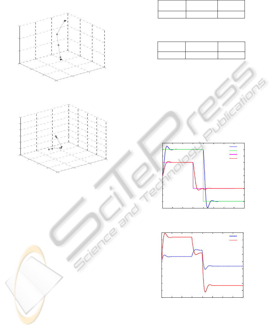
Figures 3 and 4, describe respectively the non
dominated solutions which constitute the Pareto
front for the first and the second SISO systems.
0
10
20
30
1.15
1.2
1.25
1.3
55
60
65
70
D%
Vu
Ts
i=5,i=6
i=2,i=3
i=8
i=4
i=9
i=7
i=10,i=1
Figure 3: The Pareto front for the first SISO system.
0
5
10
15
0.9
1
1.1
1.2
1.3
60
80
100
120
140
160
180
D%
Vu
Ts
i=7
i=8
i=4,i=6
i=3,i=10
i=9
i=2
i=1,i=5
Figure 4: The Pareto front for the second SISO system.
4.2 Multiobjective Predictive
Controller
To implement the controller, it is necessary to
choose a single solution among all non dominated
solutions. This choice is made by the user, if he
decides to give the priority to the minimization of
overshoot, he will choose the solution giving the
overshoot minimum value. If the most important
criterion to be minimized for the user is the settling
time, he will choose the solution giving the
minimum settling time. In this paper we choose to
make a compromise between the three closed loop
performances. For that, the step to be followed is to
calculate the norm given by (33) for every set of
i
w
and to choose the synthesis parameters
corresponding to the smallest value of
i
d .
For the first SISO system, the synthesis parameters
giving a minimal value of the norm
i
d are given in
Table 3. For the second SISO system the synthesis
parameters chosen by the supervisor are presented in
table 4. So we can notice that this proposed method
allows automatic adjusting of synthesis parameters.
Table 3: The Synthesis Parameters Chosen by the
Supervisor for the first SISO system.
p1
H
c1
H
1
ρ
2 2 7.98
Table 4: The Synthesis Parameters Chosen by the
Supervisor for the second SISO system.
p
2
H
c2
H
2
ρ
5 3 7.43
The obtained synthesis parameters, given in Table 3
and Table 4 are used with the two predictive
controllers to control the multivariable process.
The obtained results are shown in Figure 5 and
Figure 6 which respectively present the evolution of
the system outputs and the set points and the
evolution of the control signals. From these figures,
we can notice that this proposed method allows
automatic adjusting of synthesis parameters
permitting a compromise between closed loop
performances.
0 100 200 300 400 500 600 700 800
-2.5
-2
-1.5
-1
-0.5
0
0.5
1
1.5
2
2.5
y1
rc1
rc2
y2
Figure 5: Evolution of the outputs and the set points.
0 100 200 300 400 500 600 700 800
-5
-4
-3
-2
-1
0
1
2
3
4
u1
u2
Figure 6: Evolution of the control signals.
The tables 5 and 6 recapitulate respectively the
overshoots, the settling times values and the
variances of the controls found for the first and the
second SISO system.
ICINCO 2010 - 7th International Conference on Informatics in Control, Automation and Robotics
114

Table 5: Closed loop performances Values Obtained for
the First SISO System.
Overshoot
(
%
D
)
Settling
time (
s
T )
Variance of
the control
(
v
V
)
k∈ [0;400]
12 64s
0.69
k∈[401;800]
24 66s
Table 6: Closed loop Performances values for the Second
SISO System.
Overshoot
(
%
D
)
Settling
time (
s
T )
Variance of
the control
(
v
V )
k∈ [0;300]
05.8 71s
10.06
k∈[301;800]
12.8 77s
5 CONCLUSIONS
In this paper, a new method allowing the on line
adjustment of the predictive controller synthesis
parameters for multivariable systems has been
presented. The decentralized control using the
decoupling network is applied to decouple the
different subsystems and to control the MIMO
system using multiple SISO controllers. Genetic
algorithms and the weighted sum method are
exploited to find the synthesis parameters by
minimizing simultaneously three criteria which are
the overshoot, the settling time and the variance of
the control. The obtained simulation results have
shown that the proposed method can lead to
acceptable closed loop performances.
REFERENCES
Albertos, P., Sala, A., 2004. Multivariable control
systems: an engineering approach, Springer.
Bemporada, A., Muñoz de la Peñab, D., 2009.
Multiobjective model predictive control, Automatica,
vol. 45, issue 12, p. 2823-2830.
Ben Abdennour, R., Ksouri, M., Favier, G., 1998.
Application of fuzzy logic to the on-line adjustement of
the parameters of a generalized predictive controller.
Intelligent Automation and soft computing, vol.4, No
3, p.197-214.
Bouani, F., Laabidi, K., Ksouri, M., 2006. Constrained
Nonlinear Multi-objective Predictive Control, IMACS
Multiconference on "Computational Engineering in
Systems Applications"(CESA), Beijing, China, p.
1558-1565.
Bristol, E.H., 1966. On a new measure of interaction for
multivariable process control. IEEE Transactions on
control, p133-134.
Clarke, W., Mohtadi, C., Tuffs, P. S., 1987. Generalised
Predictive Control- parts I & II. Automatica, vol.23,
N° 2, p. 137-160.
Collette, Y., Siarry, P., 2002. Optimisation multiobjectif,
Editions Eyrolles.
Gambier, A., 2008. MPC and PID Control Based on
Multi-Objective Optimization. American Control
Conference, Washington, USA, p. 4727-4732.
Goldberg, D. E., 1991. Genetic Algorithms in search,
optimization and machine learning, Addison-Wesley,
Massachusetts.
Khelassi, A., Wilson, J.A., Bendib,R., 2004. Assessment of
Interaction in Process, Control Systems Dynamical
Systems and Applications Proceedings, Antalya,
Turkey, p. 463-471.
Miskovic, L., Karimi, A., Bonvin, D., Gevers, M., 2007.
Correlation-based tuning of decoupling multivariable
controllers, Automatica,
vol. 43, p. 1481-1494.
Moaveni, C., Khaki-Sedigh, A., 2006. Input-Output
Pairing based on Cross-Gramian Matrix, SICE-
ICASE International joint conference, Korea, p. 2378-
2380.
Muldera, E. F., Tiwari, P. Y., Kothare, M. V., 2009.
Simultaneous linear and anti-windup controller
synthesis using multiobjective convex optimization,
Automatica, vol.45, issue 3, p.805-811.
Popov, A., Farag, A., Werner, H., 2005. Tuning of a PID
controller Using a Multi-objective Optimization
Technique Applied to a Neutralization Plant, 44th
IEEE Conference on Decision and Control, and the
European Control Conference, Seville, Spain, p. 7139-
7143.
Richalet, J., Lavielle, G., Mallet, J., 2005. La commande
prédictive : mise en œuvre et applications
industrielles, Editions Eyrolles.
Yang, Z., Pedersen, G., 2006. Automatic Tuning of PID
Controller for a 1-D Levitation System Using a
Genetic Algorithm - A Real Case Study, IEEE
International Symposium on Intelligent Control,
Munich, Germany, p. 3098-3103.
Zalkind, C.S., 1967. Practical approach to non-
interacting control parts I and II. Instruments and
control systems, vol.40, No.3 and No.4.
DESIGN OF A MULTIOBJECTIVE PREDICTIVE CONTROLLER FOR MULTIVARIABLE SYSTEMS
115
