PARTICLE SWARM OPTIMIZATION USED FOR
THE MOBILE ROBOT TRAJECTORY TRACKING CONTROL
Adrian Emanoil Serbencu, Adriana Serbencu and Daniela Cristina Cernega
Control Systems and Industrial Informatics Department, Computer Science Faculty
"Dunarea de Jos" University from Galati, 80021 Str. Domneasca 111, Galati, Romania
Keywords: Trajectory Tracking, Nonlinear Control, Sliding Mode Control, Particle Swarm Optimization.
Abstract: The wheeled mobile robot is a nonlinear system. The trajectory tracking problem is solved using the sliding
mode control. In this paper an optimization technique is investigated in order to obtain the best values for
the sliding mode control law parameters. The performances of the control law with the optimum parameters
are analyzed in order to establish some rules. The conclusions are based on the simulation results.
1 INTRODUCTION
To solve the trajectory tracking problem for a
Wheeled Mobile Robot (WMR) it is used a
nonlinear model (Slotine and Li, 1991):
()
utxbtxfx
n
⋅+= ),(),(
(1)
where x is the state variable;
()
(
)
],,,,[
1−
=
nn
xxxxx …

;
()
n
x
is the n
th
-order derivative of x; f is a nonlinear
function; b is the gain and u is the control input.
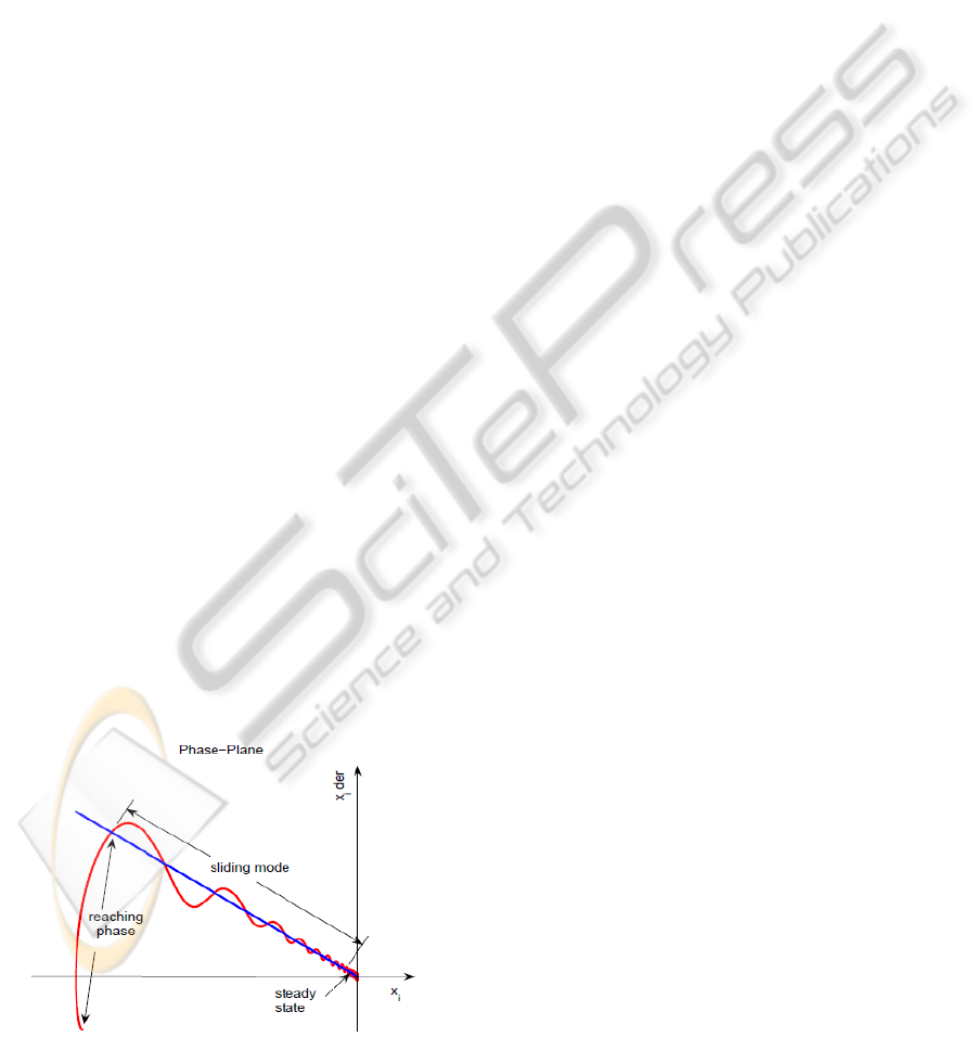
The design of a variable structure control (VSC)
(Gao and Hung, 1993) for a nonlinear system
implies two steps: (1). "reaching mode" or
nonsliding mode; (2). sliding mode.
For the reaching mode, the desired response
usually is to reach the switching manifold s,
described by:
0)( =⋅= xcxs
T
(2)
in finite time with small overshoot with respect to
the switching manifold.
The distance between the state trajectory and the
switching manifold, s is stated as:
()
0
~
,
1
=⋅
⎟
⎠
⎞
⎜
⎝
⎛
+=
−
x
dt
d
txs
n
λ
(3)
where
x
~
is the tracking error and
λ
is a strictly
positive constant which determines the closed-loop
bandwidth. For example, if n = 2,
xxs
~
~
⋅+= λ

(4)
Hence the corresponding switching manifold is
s(t)=0. For a system having m inputs, m switching
functions are needed.
It is proved that the most important virtue of the
VSC systems is robustness. Properly design of the
switching functions for a VSC system ensures the
asymptotic stability. A number of design criteria
exist for this purpose (Utkin and Young, 1978;
Dorling and Zinober, 1986). Sliding Mode is also
known to possess merits such as the invariance to
parametric uncertainties. Dynamic characteristics of
the reaching mode are very important, and this type
of control suffers from the chattering phenomenon
which is due to high frequency switching over
discontinuity of the control signal.
The parameters of the control laws have to be
positive, and their values influence the reaching rate
and the chattering. The values of these parameters
are not specified in the literature. In this paper the
optimal values for these parameters will be searched.
Many optimization methods were proposed in
literature. Recently, the Particle Swarm Optimizer
(PSO) proposed by Eberhart and Kennedy (Kennedy
and Eberhart, 1995), gained a huge popularity due to
its algorithmic simplicity and effectiveness. The
PSO is presented in Section 2. Section 3 is dedicated
to the Trajectory Tracking Problem for the WMR.
This problem is solved within the Sliding Mode
approach and the result is the sliding-mode
trajectory-tracking controller. The parameters p
i
and
q
i
of the control law are not specified in the
literature. In Section 4 PSO is used to determine the
optimal values of the control law parameters in order
to ensure maximum possible reaching rate of the
switching manifold and minimum chattering and the
results obtained are presented. Section 5 is dedicated
240
Serbencu A., Serbencu A. and Cristina Cernega D. (2010).
PARTICLE SWARM OPTIMIZATION USED FOR THE MOBILE ROBOT TRAJECTORY TRACKING CONTROL.
In Proceedings of the 7th International Conference on Informatics in Control, Automation and Robotics, pages 240-245
DOI: 10.5220/0002945702400245
Copyright
c
 SciTePress

to experimental results. Section 6 is dedicated to the
conclusion and future work directions.
2 PARTICLE SWARM
OPTIMISATION ALGORITHM
Particle swarm optimization (PSO) is one of the
evolutionary computation techniques introduced in
1995 (Kennedy and Eberhart, 1995). The algorithm
is initialized with a population of random solutions
and searches for optima by updating generations.
One entity of the population is named particle. PSO
makes use of a velocity vector to update the current
position of each particle in the swarm. Each particle
keeps track of its coordinates in the problem space
which are associated with the best solution it has
achieved so far. This value is called personal best.
The fitness value of personal best is also stored.
Another "best" position that is tracked by the
PSO is the best one, obtained so far by any particle
in the neighbours of the particle. This position is
called local best. When a particle takes all the
population as its topological neighbours, the best
position is called global best. The PSO concept
consists of, at each time step, changing the velocity
of each particle toward its personal best and local
best locations (local version of PSO). Every
component of velocity is weighted by a random
term, which assures the exploration of problem
space.
This process is iterated a set number of times, or
until a stop criterion is achieved, for example a
threshold of distance (absolute or relative) between
the two last positions, below which it is not
necessary to go. Using a population of solutions
allows PSO to avoid, in most cases, convergence to
local optimum.
Figure 1: Diagram for the concept of 3-Stages approach.
3 TRAJECTORY TRACKING
PROBLEM
In this paper the model used for the controlled robot
is a 2-order MIMO (Multiply Input Multiply Output)
nonlinear system that is "linear in control".
The model and the control law used are:
utxxBtxxfx ⋅+= ),,(),,(

(5)
),,( txxpu

=
(6)
where
[
]
n
xxxx ,,,
21
=
,
n
x ℜ∈
, f is a vector of
nonlinear functions, f
∈L
n
2
, B is a matrix of gains,
nn
B
×
ℜ∈
;
(
)
0det ≠B
; u is the control vector,
n
u ℜ∈
.
For the 2nd-order MIMO nonlinear system
having the model shown in (6) efficient sliding
mode control can be achieved via the following
stages (see Figure 1):
1
st
reaching phase motion; during this stage the
trajectory is attracted towards the switching
manifold (if the reaching condition is satisfied);
characterized by
0
~
,0
~
,0 ≠≠≠
iii
xxs

2
nd
sliding mode motion; during this stage the
trajectory stays on the switching manifold, i.e.
0
~
,0
~
,0 ≠≠=
iii
xxs

3
rd
steady state; during this stage both the state
variable and the state velocity will converge to the
steady state value, therefore:
⎪
⎩
⎪
⎨
⎧
==
→→
=
0
~
,0
~
0
~
,0
~
and,0
ii
ii
i
xx
orxx
s


The reaching law is a differential equation which
specifies the dynamics of a switching function s(x).
The differential equation of an asymptotically stable
s(x), is itself a reaching condition. In addition, by the
choice of the parameters in the differential equation,
the dynamic quality of the VSC system in the
reaching mode can be controlled.
Gao and Hung (Gao and Hung, 1993) proposed a
reaching law which directly specifies the dynamics
of the switching surface by the differential equation
)h(sPsgn(s)Qs ⋅−
⋅
−
=

(7)
where
[
]
niqqqqdiagQ
in
,,2,1,0,,,,
21
… =>=
[
] nippppdiag
in
,,2,1,0,,,,P
21
… =>=
and
(
)
])sgn(,,)sgn(,)sgn([sgn
21
T
n
ssss =
T
nn
shshshsh )](,),(),([)(
2211
=
;
,0)( >⋅ shs
ii
.0)0( =
i
h
In this paper, a constant plus proportional rate
reaching law proposed in Gao and Hung is
investigated:
(
)
sPs ⋅−⋅−= ssgnQ

(8)
PARTICLE SWARM OPTIMIZATION USED FOR THE MOBILE ROBOT TRAJECTORY TRACKING CONTROL
241

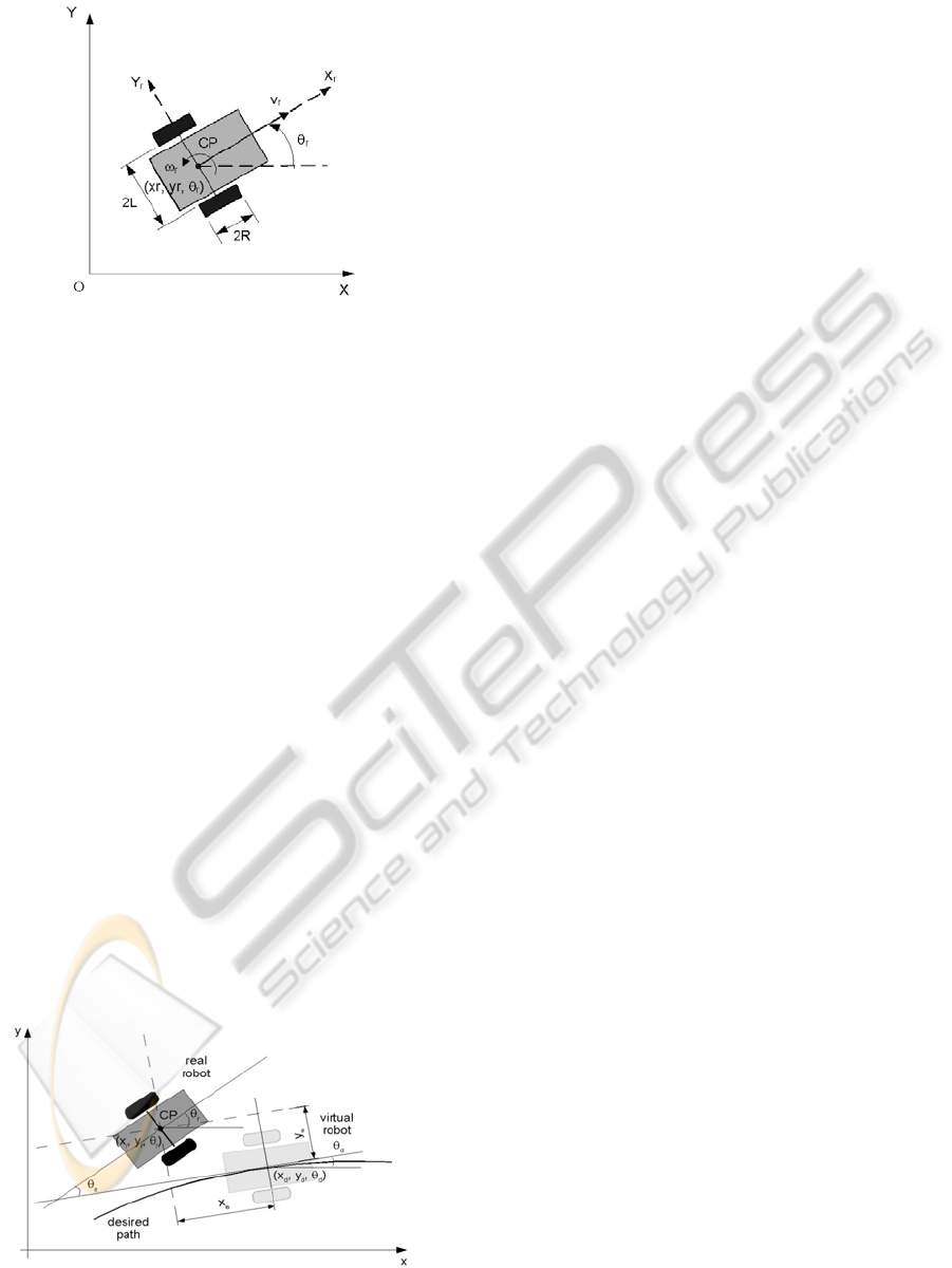
Figure 2: WMR model and symbols.
Clearly, by using the proportional rate term
sP
⋅
−
,
the state is forced to approach the switching
manifolds faster when s is large.
The purpose of the trajectory tracking is to
control the non-holonomic WMR to follow a desired
trajectory, with a given orientation relatively to the
path tangent, even when different disturbances exist.
In the case of trajectory-tracking the path is to be
followed under time constraints. Trajectory tracking
is formulated as having the WMR following a
virtual target which is assumed to move exactly
along the path with specified velocity profile.
3.1 Kinematic Model of a WMR
Figure 2 presents a WMR with two diametrically
opposed drive wheels (radius R) and free-wheeling
castors. Pr is the origin of the robot coordinates
system. 2L is the length of the axis between the drive
wheels.
ω
R
and ω
L
are the angular velocities of the
right and left wheels. Let the pose of the mobile
robot be defined by the vector,
T
rrrr
yxq ][ θ =
where
T
rr
yx ][
denotes the robot position on the plane and
θ
r
the heading angle with respect to the x-axis. In
addition, v
r
denotes the linear velocity of the robot,
and
ω
r
the angular velocity around the vertical axis.
Figure 3: Lateral, longitudinal and orientation errors
(trajectory-tracking).
For a unicycle WMR rolling on a horizontal plane
without slipping, the kinematic model can be
expressed by: which represents a nonlinear system.
⎥
⎦
⎤
⎢
⎣
⎡
⋅
⎥
⎥
⎥
⎦
⎤
⎢
⎢
⎢
⎣
⎡
=
⎥
⎥
⎥
⎦
⎤
⎢
⎢
⎢
⎣
⎡
r
10
0
0
ω
θ
θ
θ
r
r
r
r
r
r
v
sin
cos
y
x



(9)
3.2 Trajectory-tracking
Without loss of generality, it can be assumed that the
desired trajectory
T
dddd
ttytxtq )]()()([)( θ =
is
generated by a virtual unicycle mobile robot (see
Figure 3). The kinematic relationship between the
virtual configuration q
d
(t) and the corresponding
desired velocity inputs
T
dd
ttv )]()([ ω
is analogue
with (9):
⎥
⎦
⎤
⎢
⎣
⎡
⋅
⎥
⎥
⎥
⎦
⎤
⎢
⎢
⎢
⎣
⎡
=
⎥
⎥
⎥
⎦
⎤
⎢
⎢
⎢
⎣
⎡
d
10
0
0
ω
θ
θ
θ
d
d
d
d
d
d
v
sin
cos
y
x



(10)
When a real robot is controlled to move on a
desired path it exhibits some tracking error. This
tracking error, expressed in terms of the robot
coordinate system, as shown in Figure 3, is given by
⎥
⎥
⎥
⎦
⎤
⎢
⎢
⎢
⎣
⎡
⋅
⎥
⎥
⎥
⎦
⎤
⎢
⎢
⎢
⎣
⎡
−=
⎥
⎥
⎥
⎦
⎤
⎢
⎢
⎢
⎣
⎡
dr
dr
dr
dd
dd
e
e
e
-θθ
-yy
-xx
cossin
sincos
y
x
100
0
0
θθ
θθ
θ
(11)
Consequently one gets the error dynamics for
trajectory tracking as
⎪
⎩
⎪
⎨
⎧
−=
⋅−⋅=
⋅+⋅+−=
dr
d
d
ωωθ
ωθ
ωθ
e
eere
eerde
xsinvy
ycosvvx



(12)
3.3 Sliding-mode Trajectory-tracking
Control
Uncertainties which exist in real mobile robot
applications degrade the control performance
significantly, and accordingly, need to be
compensated. In this section, is proposed a sliding-
mode trajectory-tracking (SM-TT) controller, in
Cartesian space, where trajectory-tracking is
achieved even in the presence of large initial pose
errors and disturbances.
Let us define the sliding surface
T
sss ][
21
=
as
ee
xkxs ⋅
+
=
11

eeee
ysgnkykys
θ
⋅⋅
+
⋅
+
=
)(
022

(13)
where k
0
, k
1
, k
2
are positive constant, x
e
, y
e
and θ
e
are
ICINCO 2010 - 7th International Conference on Informatics in Control, Automation and Robotics
242

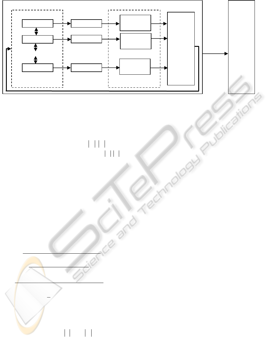
Figure 4: SM-TT controller parameters optimization with PSO.
the trajectory-tracking errors defined in (11).
If s
1
converges to zero, trivially x
e
converges to
zero. If s
2
converges to zero, in steady-state it
becomes
eeeee
ysignkyky θ ⋅⋅−⋅−= )(
0

.
For
00 >⇒<
ee
yy

if only if
ee
ykk θ /
20
⋅<
.
For
00 <⇒>
ee
yy

if only if
ee
ykk θ /
20
⋅<
.
Finally, it can be known from s
2
that convergence of
y
e
and
e
y

leads to convergence of
θ
e
to zero.
From the time derivative of (13) and using the
reaching laws defined in (8), yields:
(
)
1
spssgnqxkxs
111e1e1
⋅−⋅
−
=⋅+=

() =⋅⋅+⋅+=
eeee
ysgnkykys θ


022
(14)
(
)
2222
spssgnq ⋅−⋅−=
From (11), (12) and (14), and after some
mathematical manipulation, the output commands of
the sliding-mode trajectory-tracking controller
result:
(
)
()
()
()
e
deerde
e
dee11111
c
θcos
vθsinθvωy
θcos
ωyxkssgnqsp
v





+⋅⋅+⋅−
+
⋅−⋅−⋅−⋅−
=
(15)
()
(
)
() ()
d
e0er
erdedee22222
c
ω
ysgnkθcosv
θsinvωxωxykssgnqsp
ω +
⋅+⋅
⋅−⋅+⋅+⋅−⋅−⋅−
=

Let us define
ss
T
⋅⋅=
2
1
V
as a Lyapunov function
candidate, therefore its time derivative is
=⋅−⋅−⋅+
+⋅−⋅−⋅=⋅+⋅=
))sgn(spsq(s
))ssgn(psq(sssss
22222
111112211


V
s2pspsQs
211
T
⋅−⋅−⋅⋅=
For
V

to be negative semi-definite, it is sufficient to
choose
q
i
and p
i
such that q
i
, p
i
≥ 0.
But the optima values for
q
i
, p
i
≥ 0 will be
determined in the next section.
The
signum functions in the control laws were
replaced by
saturation functions, to reduce the
chattering phenomenon (Slotine and Li, 1991).
4 SLIDING MODE
CONTROLLER PARAMETERS
EVALUATED WITH PSO
Solving the Trajectory Tracking Problem with a
SMC, leads to the reaching laws (15). In literature,
the parameters
q1, q2, p1 and p2 are usual
determined through experiments (Solea and
Cernega, 2009) and have great impact on the
performance of the controller.
q1, q2 influence the
rate at which the switching variable
s(x) reach the
switching manifold
S. Parameters p1, p2 force the
state
x to approach the switching manifolds faster
when
s is large.
Choosing parameters through experiments only
depends on experience or repeated debugging. In
this paper is presented a method of choosing the
parameters of the Sliding Mode Controller using the
PSO algorithm. The advantages of PSO are:
simplicity and efficiency, proven in many other
parameters training problems (Mendes
et al., 2002;
Kim et al., 2008). The optimisation algorithm is
working off-line. The
P and Q parameters found by
PSO can be used in real-time implementation of
SM-TT controller on PatrolBot Robot (see Figure 4).
PSO algorithm is generating, at each step, a
number of solutions equal to the number of particles.
The quality (fitness) of the solutions is evaluated
with the objective function. PSO algorithm requires
current solutions fitness to calculate new solutions at
the next iteration. The objective function used in
PSO takes into account booth the speed of reaching
Evaluate
Solution 1
Evaluate
Solution n
Particle 1
Particle 2
Particle n
…
Solution 1
Solution 2
Solution n
…
Particle Communicate
whith their Neighbors
Evaluate
Solution 2
…
Runing Simulink Schema
and Evaluate Solution
Updating
personal
best
position
AND
Updating
global
best
position
OFFLINE OPTIMIZATION
Realtime
SlidingMode
Controller
Optimal
Parameters
PARTICLE SWARM OPTIMIZATION USED FOR THE MOBILE ROBOT TRAJECTORY TRACKING CONTROL
243

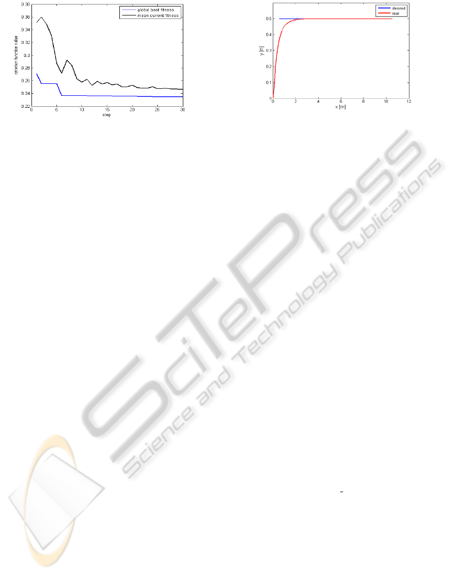
Figure 5: The evolution of best value found by PSO and of
the mean criterion function over all particle.
manifolds and the amplitude of the chattering. This
is accomplished using the sum of root mean square
of the two errors
x
e
and y
e
(11). The evaluation of
every set of parameters is achieved after running a
numerical simulation of the SM-TT control structure
implemented in a Matlab Simulink schema that
contains the model of the robot.
The horizon of simulation and initial conditions
are chosen to allow a correct comparison between
sets of parameters. The step of simulation is selected
according to the one used to control the PatrolBot.
Let us suppose that the swarm is composed by
n particles. Each particle i is recorded as a structure
that transfer from the current iteration
t to the next
iteration the four elements specified below:
• The current position of i
th
particle in the
search space at the moment
t is given through a
vector with 4 components
x
i
(t)=(x
q1i
(t), x
q2i
(t), x
p1i
(t), x
p2i
(t)).
• The current velocity v
i
(t) of i particle is a
vector with components for each direction of the
search space too.
• The best position found up to now by this
particle is given by a vector
l
i
(t) with the same
meaning as
x
i
(t).
• The quality of personal best position l
i
(t).
In order to compute the next position where to
move, every particle of the swarm needs one more
information: the best position found by its
neighbours stored in the vector
g
i
(t). Generally, this
is written simply
x, v, l, and g. The d
th
component of
one of these vectors is indicated by the index
d, for
example
x
d
. With these notations, the motion
equations of a particle are, for each dimension
d ∈ { q1i, q2i, p1i, p2i}:
⎩
⎨
⎧
+←
−+−+←
ddd
dddddd
vxx
xgcxlcvcv )()(
321
(16)
The confidence coefficients are defined as
Figure 6: Simulated trajectory with the parameters value
found by PSO. Experimental SM-TT control starting from
an initial error state (x
e
(0) = -0.5, y
e
(0) = -0.5, θ
e
(0) = 0).
follows:
• c
1
is (confidence in its own movement) the
• inertia weight, with linear variance from 0.9
to 0.4.
• c
2
, c
3
(respectively confidence in its best
performance and that of its best informant) are
randomly selected at each step according to an
uniform distribution in the interval [0,
c
max
].
A circular neighbourhood is used as graph of
influence.
5 EXPERIMENTAL RESULTS
Based on the above analysis, mathematical
simulation software MATLAB was used to
accomplish the experiment simulation study.
The mobile robot PatrolBot used in simulation is
assumed to have the same structure as in Figure 2.
Parameter values of the PatrolBot are: mass of the
robot body 46 [Kg], radius of the drive wheel
0.095 [m], and distance between wheels 0.48 [m].
The parameters of sliding modes were held constant
during the experiments:
k
1
= 0.75, k
2
= 3.75, and
k
0
= 2.5; and the desired trajectory is given by
v
d
= 0.5 [m/s], ω
d
= 0 [rad/s].
The experiments were done on the robot with the
initial error (
x
e
= -0.5 [m], y
e
= -0.5 [m], θ
e
= 0 [deg])
and used the reaching law (8).
Settings, used in Matlab implementation of PSO
algorithm, are: particle number
n = 20; maximal
number of iteration = 30,
c
max
=1.9. The criterion
function used for solution evaluation are the sum of
root mean square (RMS) of the two errors
longitudinal -
x
e
and lateral - y
e.
RMS error is an old,
proven measure of control and quality. Taking into
account that parameters must be positive and value
too large can causes chattering, the search interval
for each SM parameters was selected to be [0.01 5].
In Figure 5 the evolution of criterion function
ICINCO 2010 - 7th International Conference on Informatics in Control, Automation and Robotics
244

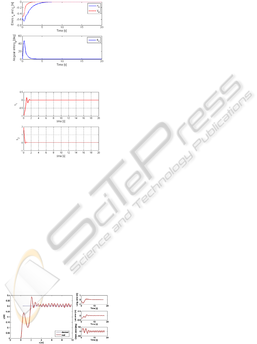
Figure 7: Longitudinal, lateral and orientation errors for
experimental SM-TT control.
Figure 8: Sliding surface for SM-TT controller.
best value found by PSO is presented. Average value
of criterion function for all particles is also recorded.
Note that a number of 15 iterations are sufficient to
find a good set of values of parameters.
The parameters values for the considered
PatrolBot, found by PSO are
q1=0.4984, q2=1.9075,
p1=1.0230 and p2=2.4872.
In Figures 6 and 7, the simulation results for the
case of optimised parameters are presented.
In Figure 8 the two sliding manifolds are
represented. In Figure 8 one can also see the value of
the reaching time.
Figure 9 presents the response of the robot
corresponding to the situation of a poor choice of the
control law parameters without any optimisation.
It is easy to see the difference between the
performances between Figures 6 and 9.
Figure 9: An unfavourable case of experimental SM-TT
control.
6 CONCLUSIONS
The paper proposed an efficient method to determine
the optimum set of parameters for the sliding mode
controller. The PSO algorithm proved to be adequate
for this problem because it eliminates the need for
repeated simulations in order to find a satisfactory
set of parameters. The tests have proven that this
optimization technique is efficient for the problem to
be solved. A very good solution without chattering
was found in a quite acceptable time interval and
number of iterations.
The search of the optimum values for the sliding
mode trajectory tracking control laws parameters
was done in order to use, in the future, such
optimum parameters into a supervised control
structure having the ability to switch between
different controllers.
ACKNOWLEDGEMENTS
This work was supported by the CNCSIS -
UEFISCSU, project number IDEI-506/2008.
REFERENCES
Slotine, J., Li, W., 1991. Applied Nonliner Control,
Prentice Hall, New Jersey.
Gao, W., Hung, J., 1993. Variable structure control of
nonlinear systems: A new approach. IEEE
Transactions on Industrial Electronics, 40, pp. 45–55.
Utkin, V., Young, K., 1978. Methods for constructing
discontinuity planes in multidimensional variable
structure systems. Automation and Remote Control,
39, pp. 1466–1470.
Dorling, C., Zinober, A., 1986. Two approaches to
hyperplane design in multivariable variable structure
control systems. Int Journal Control, Vol. 44, p.65–82
Kennedy, J., Eberhart, R. C., 1995. Particle Swarm
Optimization. IEEE International Conference on
Neural Networks, Perth, Australia, pp. 1942-1948.
Solea, R., Cernega, D. C., 2009. Sliding Mode Control for
Trajectory Tracking Problem - Performance
Evaluation. Artificial Neural Networks – ICANN 2009,
Lecture Notes in Computer Science, Vol. 5769, pp.
865-874.
Mendes, R., Cortez, P., Rocha, MR., Firns, J., 2002.
Particle Swarms for Feedforward Networks Trening.
International Conference on Neural Networks,
Honolulu (Hawaii), USA, pp. 1895-1889.
Kim, T. H., Maruta, I., Sugie, T., 2008. Robust PID
controller tuning based on the constrained particle
swarm optimization. Automatica, Vol. 44, pp. 1104–
1110.
PARTICLE SWARM OPTIMIZATION USED FOR THE MOBILE ROBOT TRAJECTORY TRACKING CONTROL
245