
SIMPLE DERIVATION OF A STATE OBSERVER OF LINEAR
TIME-VARYING DISCRETE SYSTEMS
Yasuhiko Mutoh
Department of Applied Science and Engineering, Sophia University, 7-1, Kioicho, Chiyoda-ku, Tokyo, Japan
Keywords:
Pole Placement, State Observer, Linear Time-Varying System, Discrete System.
Abstract:
In this paper, a simple calculation method to derive the Luenberger observer for linear time-varying discrete
systems is presented. For this purpose, the simple design method of the pole placement for linear time-varying
discrete systems is proposed. It is shown that the pole placement controller can be derived simply by finding
some particular ”output signal” such that the relative degree from the input to this new output is equal to the
order of the system. Using this fact, the feedback gain vector can be calculated directly from plant parameters
without transforming the system into any standard form.
Then, this method is applied to the design of the observer, i.e., because of the duality of linear time-varying
discrete system, the state observer can be derived by simple calculations.
1 INTRODUCTION
The design of the state observer for linear time-
varying discrete systems is well established. As for
the continuous case, the condition for a system to be
a state observer is very simple. However, different
from the time-invariant case, calculation procedure to
obtain the observer gain is not straightforward. This
paper gives a simple calculation method to design
the state observer for linear time-varying discrete sys-
tems.
Since the design of the observer is based on
the pole placement technique, simplified calculation
method to derive the pole placement feedback gain
vector for linear time-varying discrete systems is con-
sidered first. We define the pole placement of lin-
ear time-varying discrete systems as follows. The
problem is to find a time-varying state feedback gain
for linear discrete time-varying discrete system, so
that the closed loop system is equivalent to the time-
invariant system with desired poles.
Usually, the pole placement design procedure
needs the change of variable to the Flobenius stan-
dard form, and hence, is very complicated. To sim-
plify this procedure, it will be shown that the pole
placement controller can be derived simply by find-
ing some particular ”output signals” such that the rel-
ative degree from the input to this output is equal to
the order of the system [4]. Using this fact, the feed-
back gain vector can be calculated directly from plant
parameters without transforming the system into any
standard form.
Because of the duality of the linear discrete time-
varying system, the simplified pole placement tech-
nique can be applied to thedesign of the state observer
for linear discrete time-varying discrete systems.
In the sequel, the simple pole placement technique
is proposed in Section 2, and then, this method is used
to the observer design problem in Section 3.
2 POLE PLACEMENT OF
LINEAR DISCRETE
TIME-VARYING SYSTEMS
Consider the following linear time-varying discrete
system with a single input.
x(k+ 1) = A(k)x(k) + b(k)u(k) (1)
Here, x ∈ R
n
and u ∈ R
1
are the state variable and
the input signal respectively. A(k) ∈ R
n×n
and b(k) ∈
R
n
are time-varying parameter matrices. The problem
is to find the state feedback
u = h
T
(k)x(k) (2)
which makes the closed loop system equivalent to
the time invariant linear system with arbitrarily stable
poles.
30
Mutoh Y. (2010).
SIMPLE DERIVATION OF A STATE OBSERVER OF LINEAR TIME-VARYING DISCRETE SYSTEMS.
In Proceedings of the 7th International Conference on Informatics in Control, Automation and Robotics, pages 30-34
DOI: 10.5220/0002945800300034
Copyright
c
SciTePress

Definition 1. The system (1) is called completely
reachable in step n from the origin, if for any x
1
∈ R
n
,
there exists a finite input u(m) (m = k, ··· , k + n − 1)
such that x(k) = 0 and x(k+ n) = x
1
.
Lemma 1. The system (1) is completely reachable in
step n from the origin, if and only if
rank [ b(k+ n− 1),Φ(k+ n, k+n−1)b(k+ n− 2),
··· ,Φ(k+n, k + 1)b(k) ]
= rank U
R
(k) = n,
∀
k (3)
where Φ(i, j) is the transition matrix from k = j to k = i,
i.e.,
Φ(i, j) = A(i− 1)A(i− 2)··· A( j) i > j (4)
∇∇
Now, consider the problem of finding a new output
signal y(k) such that the relative degree from u(k) to
y(k) is n. Here, y(k) has the following form.
y(k) = c
T
(k)x(k) (5)
Then, the problem is to find a vector c(k) ∈ R
n
that
satisfies this condition.
Lemma 2. The relative degree from u to y defined by
(5) is n, if and only if
c
T
(k+ 1)b(k) = 0
c
T
(k+ 2)Φ(k+ 2, k + 1)b(k) = 0
.
.
. (6)
c
T
(k+ n− 1)Φ(k+ n − 1, k+ 1)b(k) = 0
c
T
(k+ n)Φ(k+ n, k + 1)b(k) = 1
(Here, c
T
(k + n)Φ(k+ n, k+ 1)b(k) = 1 without loss
of generality.) ∇∇
Proof : This is obvious by checking y(k + 1), ···,
y(k+ n).
If the system (1) is completely reachable in step n,
there exists a vector c(k) such that the relative degree
from u(k) to y(k) = c
T
(k)x(k) is n. And, from (6),
such a vector, c(k), is obtained by
c
T
(k) = [0, · · · , 0, 1] [ b(k − 1), Φ(k, k − 1)b(k−2),
··· , Φ(k, k + 1− n)b(k− n) ]
−1
= [0, 0, · ·· , 1]U
−1
R
(k− n) (7)
The next step is to derive the state feedback for the
arbitrary pole placement.
The new output, y(k) = c
T
(k)x(k), with c(k) ob-
tained by (7), satisfies the following equations.
y(k) = c
T
(k)x(k)
y(k+ 1) = c
T
(k+ 1)Φ(k+1, k)x(k)
.
.
. (8)
y(k+ n− 1) = c
T
(k+ n− 1)Φ(k+n−2, k)x(k)
y(k+ n) = c
T
(k+ n)Φ(k+n−1, k)x(k) +u(k)
Let q(z) be a desired stable polynomial of z-
operator, i.e.,
q(z) = z
n
+ α
n−1
z
n−1
+ ··· + α
0
(9)
By multiplying y(k + i) by α
i
(i = 0, ··· ,n − 1) and
then summing them up, the following equation is ob-
tained from (8).
q(p)y(k) = d
T
(k)x(k) + u(k) (10)
where d(k) ∈ R
n
is defined by the following.
d
T
(k) = [ α
0
, α
1
, ··· , α
n−1
, 1 ]
×
c
T
(k)
c
T
(k+ 1)Φ(k+ 1, k)
.
.
.
c
T
(k+ n)Φ(k+ n, k)
(11)
Hence, the state feedback,
u = −d
T
(k)x(k) + r(k) (12)
makes the closed loop system as follows.
q(z)y(k) = r(k) (13)
where r(k) is an external input signal.
This control system can be summarized as fol-
lows. The given system is
x(k+ 1) = A(k)x(k) + b(k)u(k) (14)
and, using (4), (9), and (11) the state feedback for the
pole placement is given by
u(k) = −d
T
(k)x(k). (15)
Then, the closed loop system becomes
x(k+ 1) = (A(k) − b(k)d
T
(k))x(k). (16)
Let T(k) be the time varying matrix defined by
T(k) =
c
T
(k)
c
T
(k+ 1)Φ(k+ 1, k)
.
.
.
c
T
(k+ n− 1)Φ(k+ n − 1, k)
(17)
and define the new state variable w(k) by the follow-
ing equations.
x(k) = T(k)w(k), w =
y(k)
y(k+ 1)
.
.
.
y(k+ n− 1)
(18)
SIMPLE DERIVATION OF A STATE OBSERVER OF LINEAR TIME-VARYING DISCRETE SYSTEMS
31

Using the above, (16) is transformed into
w(k+ 1)
= T
−1
(k+ 1)(A(k) − b(k)d
T
(k))T(k)w(k)
=
0 1 ··· 0
.
.
.
.
.
.
.
.
.
.
.
. 1
−α
0
··· ··· −α
n−1
w(k)
= A
∗
w(k) (19)
This implies that the closed loop system is equiv-
alent to the time invariant linear system which has the
desired closed loop poles (det(zI − A
∗
) = q(z)).
Theorem 2. If the system (1) is completely reachable
in step n, then, the matrix for the change of variable,
T(k), given by (17) is nonsingular for all k. ∇∇
Example 1.
Consider the following unstable system.
x(k+ 1) = A(k)x(k) + b(k)u(k) (20)
where
A(k) =
1 2+ cos0.1k
2+ sin0.2k 2
b(k) =
0
1
(21)
From (7), c
T
(k) is obtained as follows.
c
T
(k) = [ 0, 1 ][ b(k− 1), A(k− 1)b(k− 2) ]
−1
=
1
2+ cos0.1(k− 1)
0
(22)
The purpose is to design the state feedback so that the
closed loop system is equivalent to the linear time in-
variant system with λ
1
= 0.4 and λ
2
= 0.5 as its closed
loop poles. This implies that the desired closed loop
characteristic polynomial is
q(z) = z
2
+ 0.9z+ 0.2.
From (11),
d
T
(k) = [ 0.2, 0.9, 1 ]
×
c
T
(k)
c
T
(k+ 1)A(k)
c
T
(k+ 2)A(k+ 1)A(k)
=
d
1
(k) d
2
(k)
(23)
In the above, d
1
(k) and d
2
(k) are given by
x
x
1
2
0
10
20
-10
-20
Figure 1: Responce of the state variable (x) of the system.
d
1
(k) =
0.2
γ(k− 1)
+
0.9
γ(k)
+
1
γ(k+ 1)
+ 2+ sin0.2k
d
2
(k) = 0.9+
γ(k)
γ(k+ 1)
+ 2
where
γ(k) = 2+ cos0.1k
Fig.1 shows the simulation results.
3 STATE OBSERVER
In this section, we consider the design of the observer
for the following linear time-varying system.
x(k+ 1) = A(k)x(k) + b(k)u(k)
y(k) = g
T
(k)x(k) (24)
Here, y(k) ∈ R is the output signal of this system.
The problem is to design the full order state observer
for (24). Consider the following system as a candidate
of the observer.
ˆx(k+ 1) = F(k) ˆx(k) + b(k)u(k) + h(k)y(k)
= F(k) ˆx(k) + b(k)u(k) + h(k)g
T
(k)x(k)
(25)
where F(k) ∈ R
n×n
, and h(k) ∈ R
n
. Define the state
error e(k) ∈ R
n
by
e = x(k) − ˆx(k) (26)
Then, e(k) satisfies the following error equation.
e(k+ 1) = F(k)e(k) + (A(k) − F(k)
−h(k)g
T
(k))x(k) (27)
Hence, (25) is a state observer of (24) if F(k) and
h(k) satisfy the following condition.
F(k) = A(k) − h(k)g
T
(k) (28)
F(k) : arbitrarily stable matrix
Then, the problem is to find h(k) such that F(k)
is equevalent to a constant matrix F
∗
with arbitrar-
ily stable poles. Consider the pole placement control
problem of the following system.
w(k+ 1) = A
T
(−k)w(k) + g(−k)v(k) (29)
ICINCO 2010 - 7th International Conference on Informatics in Control, Automation and Robotics
32

where w(k) ∈ R
n
and v(k) ∈ R
1
are the state variable
and an input signal.
Let Ψ(i, j) be the state transient matrix of the sys-
tem (29). Then, we have the following relation.
Φ
T
(i, j) = Ψ(− j, −i) (30)
Definition 2. The system (24) is called completely
obsermable in step n, if from y(k), y(k+ 1), ···, y(k+
n− 1), the state, x(k), can be determined uniquely for
any k.
Lemma 3. The system (24) is completely observable
in step n, if and only if
rank
g
T
(k)
g
T
(k+ 1)Φ(k+ 1, k)
.
.
.
g
T
(k+ n− 1)Φ(k+ n − 1, k)
= rank U
o
(k) = n, ∀k (31)
From the property of the duality of the time vary-
ing discrete system, if the pair (A(k), g
T
(k)) is com-
pletely observable in step n, the pair (A
T
(−k), g(−k))
is completely reachable in step n. Then, if the pair
(A(k), g
T
(k)) is completely observable in step n, the
system (29) has a state feedback
v(k) = h
T
(−k)w(k) (32)
such that the closed loop system is equevalent to the
linear time invariant system with arbitrarily stable
poles.
This implies that for some state transformation
matrix, P(−k) ∈ R
n
,
P
−1
((k+ 1))(A
T
(−k) − g(−k)h
T
(−k))P(k)
= F
∗T
(33)
where, F
∗T
is a constant matrix with arbitrarily stable
poles. From this and the duality, we have the follow-
ing equation.
P
−1
(−k)(A(k) − h(k)g
T
(k))P(−(k+ 1))
= F
∗
(34)
Hence, using this h(k), the state observer for the
system (24) is obtained.
Example 2.
Consider the following system.
x(k+ 1) = A(k)x(k) + b(k)u(k)
y(k) = g
T
(k)x(k) (35)
where
A(k) =
0 1
−0.7 −(1.2 + 0.5cos0.4k)
b(k) =
1
1
, g
T
(k) = [ 2, 1 ] (36)
The dual system matrices are as follows.
A
T
(−k) =
0 −0.7
1 −(1.2+ 0.5cos0.4(−k))
g(−k) =
2
1
(37)
From (7), c
T
(−k) for the new output matrix is ob-
tained as
c
T
(−k) = [ 0, 1 ][ g(−(k− 1)),
A
T
(−(k− 1))g(−(k− 2)) ]
−1
=
1
γ(−(k− 1))
−1 2
(38)
where,
γ(−k) = 4.7− 2λ(k)
λ(k) = 1.2+ 0.5cos0.4k. (39)
The purpose is to design the state feedback so that
the closed loop system is equivalent to the linear time
invariant system with λ
1
= 0.3 and λ
2
= 0.4 as its
closed loop poles. This implies that the desired closed
loop characteristic polynomial is
q(z) = z
2
+ 0.7z+ 0.12.
From (11), d
T
(−k) is calculated as follows.
d
T
(−k) = [ 0.12, 0.7, 1 ]
×
c
T
(−k)
c
T
(−(k+ 1))A(−k)
c
T
(−(k+ 2))A(−(k + 1))A(−k)
=
d
1
(−k) d
2
(−k)
(40)
Here, d
1
(k) and d
2
(k) are
d
1
(k) = −
0.12
γ(k− 1)
+
0.7
γ(k)
+
1
γ(k+ 1)
(0.2− λ(k+ 1))
d
2
(k) =
0.12
γ(k− 1)
+
0.7
γ(k)
(0.2− λ(k))
+
1
γ(k+ 1)
{−0.2− (0.2+ λ(k+ 1))λ(k)}
SIMPLE DERIVATION OF A STATE OBSERVER OF LINEAR TIME-VARYING DISCRETE SYSTEMS
33
x
x
1
1
^
0
2
4
6
-2
-4
-6
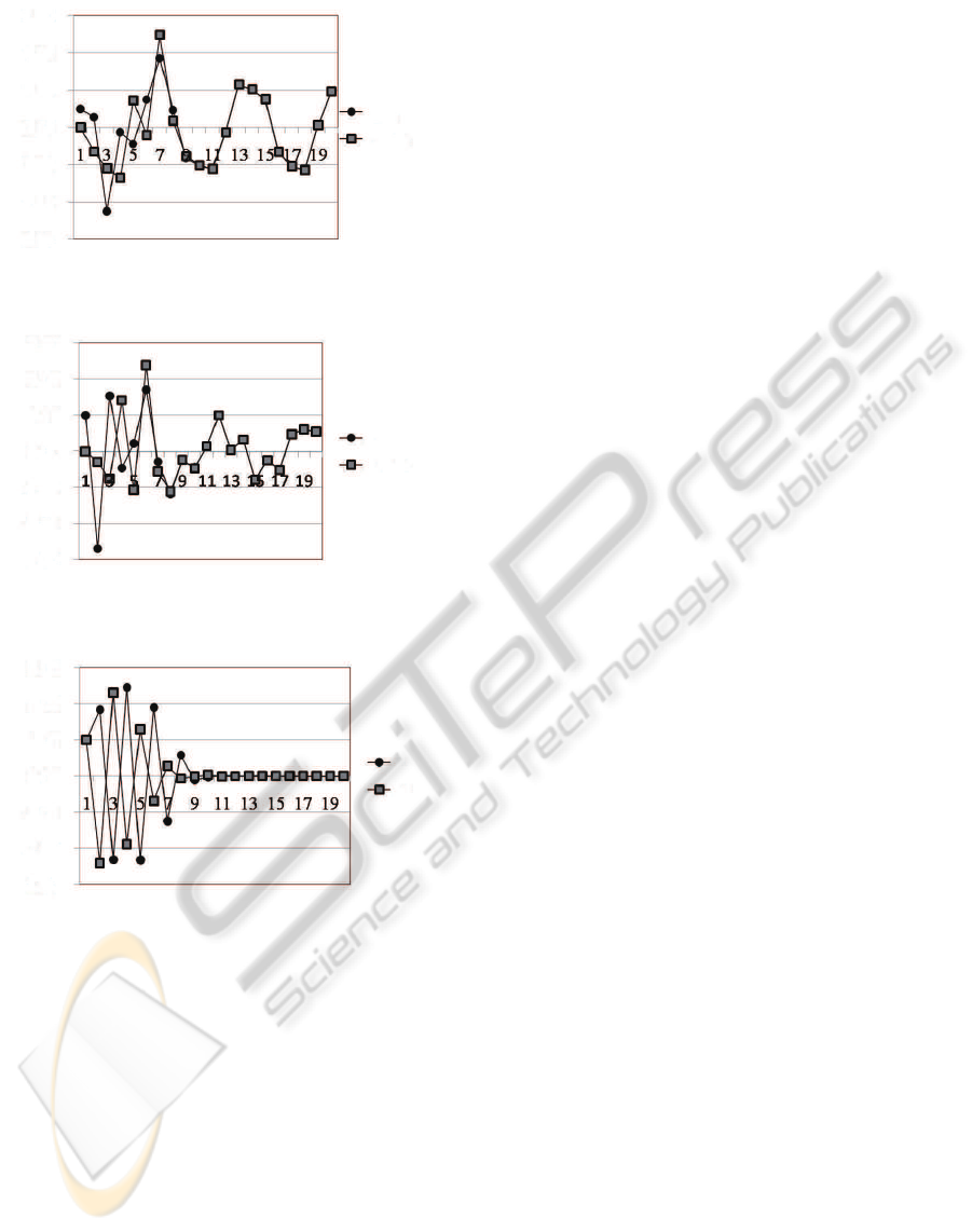
Figure 2: Responce of x
1
(k) and ˆx
1
(k).
x
x
^
2
2
1
2
3
-1
-2
-3
0
Figure 3: Responce of x
2
(k) and ˆx
2
(k).
e
e
1
2
0
2
3
-1
-2
-3
1
Figure 4: Responce of the estimation error (e
1
(k) = x
1
(k)−
ˆx
1
(k), e
2
(k) = x
2
(k) − ˆx
2
(k)).
Hence, the observer gain vector, h(k), is obtained as
h(k) = −d(k) (41)
and, using this h(k), the observer is
ˆx(k+ 1) = {A(k) − h(k)g
T
(k)} ˆx(k)
+b(k)u(k) + h(k)y(k) (42)
Fig.2 ∼ 4 show the simulation results with u(k) =
2cos(0.9k). The initial condition of the plant is
x
1
(1) = x
2
(1) = 1.
4 CONCLUSIONS
In this paper, a simple design method for the state
observer for linear time-varying discrete systems is
proposed. We first proposed the simple derivation
method of the pole placement state feedback gain for
liner time-varying discrete system. Feedback gain can
be calculated directly from the plant parameters with-
out the transformation of the system into any standard
form, which makes the design procedure very sim-
ple. This technique is applied to the observer design
procedure using the duality of the linear time-varying
system. The author appreciates the helpful comments
of the anonymous reviewers.
REFERENCES
Kwakaernaak H. C., Linear Optimal Control Systems.
Wiley-Interscience, 1972
Chi-Tsong Chen C., Linear System Theory and Design
(Third edition). Oxford University Press, 1999
T. Kailath C., Linear Systems. Prentice-Hall, 1980
Tse E., and Athans M., Optimal Minimal-Order Observer-
Estimators for Discrete Linear Time-Varying System.
IEEE, Transaction on AC, AC-15, 4, 416–426, 1970
Mutoh Y, Simple Design of the State Observer for Linear
Time-Varying Systems. 6-th ICINCO, 2009
ICINCO 2010 - 7th International Conference on Informatics in Control, Automation and Robotics
34
