
EFFICIENT LOCOMOTION ON NON-WHEELED
SNAKE-LIKE ROBOTS
Julián Colorado, Antonio Barrientos, Claudio Rossi, Mario Garzón, María Galán and Jaime del Cerro
Robotics and Cybernetics Group, Robotics and Automation Center UPM-CSIC, Universidad Politécnica de Madrid, Spain
Keywords: Serpenoid curves, Snake bio-mechanisms, Bio-inspired locomotion, Crawling robots.
Abstract: This article presents our current work on studying energy efficient locomotion on crawling snake-like
robots. The aim of this work is to use existing biological inspired methods to demonstrate lateral undulation
planar gaits for efficiently controlling high-speed motion as a function of the terrain surface. A multilink
non-wheeled snake-like robot is being developed for experimentation and analysis of efficient serpentine
locomotion based on simulation results.
1 INTRODUCTION
In nature, snakes are able to move on different
environments. Generally speaking, snakes can adapt
to a particular terrain employing changes in their
muscles-shape (Kane and Lecision, 2000). This
potential provides snakes with higher rough terrain
adaptability on irregular surfaces compared to
legged animals.
The first attempts of approaching biological
inspired snake motion using an artificial counterpart
was conducted by Hirose in the 70’s (Hirose, 1993).
He made the analysis of limbless motions
experimental data and suggested mathematical
description of the snake’s instant form. The curve
was called –serpenoid– and is widely used for the
snake robot’s control assignment nowadays. The
first designs of Hirose’s snake robots had modules
with small passive wheels, and since then, most of
the current developments (Downling, 1997),
(Chirikjian and Burdick, 1990), (Ostrowski, 1995)
remain using snake robots with wheels in order to
facilitate forward propulsion. Nonetheless, snake-
like robots that have no wheels are closer to their
biological counterparts. The difficulty in analyzing
and synthesizing snake locomotion mechanisms is
not as simple as wheeled mechanisms. One of the
main drawbacks relies on their poor power
efficiency for surface traction, and consequently
locomotion. While most works address contributions
in terms of snake control and full autonomous
navigation (Kamegawa et al., 2002), (Prautsch and
Mita, 1996), (Transeth et al., 2006) our work is
focused on providing modeling foundations to use a
non-wheeled snake robot that can adapt to the
environment at the advantage of energy efficiency.
Our goal is to establish a mathematical
framework for modeling that relates the existing
knowledge of biological snake locomotion with the
dynamics behavior that achieves minimal energy
waste when the snake moves at high speeds over
1m/s. Section 2 of this article briefly presents how to
achieve lateral undulation serpentine gaits using
Hirose’s serpenoid curves and how to integrate that
approach within the dynamics equations of motion.
A friction model is also addressed in order to
achieve the proper forward motion based on internal
joint torques. Section 3 introduces how to optimize
snake locomotion by choosing the optimal serpenoid
curve parameters that minimize energy
consumption. Simulation results show efficient
motion over ground. Finally, Section 4 presents
conclusions and upcoming future work will present
experimental validation using an experimental
testbed (under current development) that consists on
nine articulated modules serially connected.
2 SERPENTINE MODELING
Almost all limbless vertebrates, including snakes,
mimic their ancestors by shaping their bodies in a
–S-shaped– curve that travels tailwards (Gray and
Lissmann, 1950). Snakes commonly propel
themselves on the ground or water by summing
246
Colorado J., Barrientos A., Rossi C., Garzón M., Galán M. and del Cerro J. (2010).
EFFICIENT LOCOMOTION ON NON-WHEELED SNAKE-LIKE ROBOTS.
In Proceedings of the 7th International Conference on Informatics in Control, Automation and Robotics, pages 246-251
DOI: 10.5220/0002945902460251
Copyright
c
SciTePress
longitudinal resultants of lateral forces. This kind of
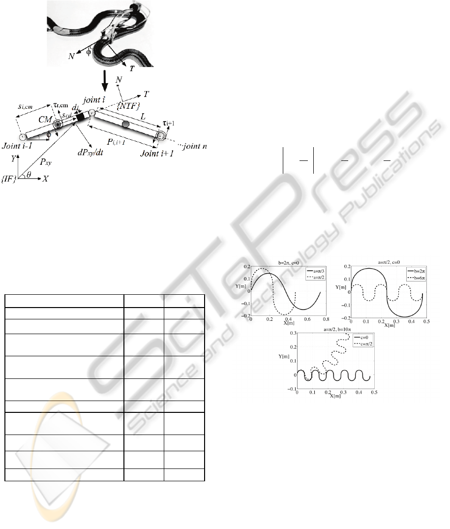
motion is called Lateral Undulation (see Figure 1).
Figure 1: (Above): The s-shape that biological snakes
perform to move forward using lateral undulation pattern.
(Below): serially coupled rigid body system description.
Table 1 introduces a description of the variables
involved within the framework of snake-like robot
modeling based on Figure 1.
Table 1: Description of snake-like robot parameters.
Description
Notation Units
Number of links
n
-
Joint position at body-i
i
φ
[rad]
Body-i orientation with respect to
inertial frame {IF}
i
θ
[rad]
Vector position from joint’s
frame to body’s CM
cmi
s
,
[m]
Distance from body’s CM to
differential length
d
L
cd
s
[m]
Link-i length
L
[m]
Vector position from joint-i frame
to joint i+1
1, +ii
p
[m]
Joint torque of body-i
i
τ
[Nm]
Friction torque of body-i CM
cmr,
τ
[Nm]
Friction coefficients
TN
CC ,
[s
-1
]
2.1 Serpenoid Curves
Hirose found that snakes take their body onto
so-called serpenoid curve when they move with a
serpentine gait. Considerer the snake-like robot
depicted in Figure 1, which consist on n-links
serially connected through n-1 joints. The
undulatory motion of a snake can be imitated by
changing the relative angles
φ
of snake’s bodies as
shown in Equation 1. See details in (Hirose and
Morishima, 1990).
φ
i
(
t
) = 2
α
sin
ω
s
t
+ (
i
−1)
β
( )
+
γ
(1)
The term
φ
i
(
t
)
is a sinusoidal function varying
along the arc length
i
/
n
∀
i
:
i
= 1...
n
−1
( )
at
ω
s
angular speed propagation. The terms,
α
,
β
and
γ
are the parameters that determine the shape of the
serpentine curve realized by the snake-like robot
(e.g. if
γ
= 0
, the curve will describe a straight path
and when
γ
≠ 0
the curve will trace a circular path).
Equation 2 shows these parameters.
α
=
a
sin
β
2
,
β
=
b
n
,
γ
= −
c
n
(2)
Based on different choices of the parameters
a
,
b
and
c
, Figure 2 shows several serpenoid curves
profiles. The parameter
a
determines the degree
undulation,
b
the number of periods in a unit length,
and
c
is the motion circular bias.
Figure 2: Computing Lateral Undulation serpentine gaits
using serpenoid curves.
Our first objective is to merge this serpentine
curve approach into our snake dynamics model. The
key property of snakes in achieving forward
locomotion is the difference in the friction
coefficients for the tangential–T and the normal–N
directions with respect to the body. In particular, the
normal friction tends to be much larger than the
tangential friction, leading to avoidance of side
slipping. In order to analyze such property, next
subsection introduces the solution of the dynamic’s
Equations of Motion –EoM of a multilink articulated
body system as shown in Figure 1, and the
EFFICIENT LOCOMOTION ON NON-WHEELED SNAKE-LIKE ROBOTS
247

incorporation of a simple friction model to provide
accurate snake forward propulsion.
2.2 Snake-Like Robot Dynamics
Applying the D'Alembert's principle (Fu et al., 1987)
and assuming a snake’s tail (base) to end-body
(head) recursive propagation of kinematics spatial
velocities in (3) [angular and linear components
stacked in a single 6-dimensional quantity]:
{ }
niHVRPV
iiii
T
ii
T
iii
...1:
11,,1
=∀+=
−−−
φ
(3)
In multibody dynamics, spatial quantities must
be propagated and projected onto unique frames in
order to be operator on. For this purpose, operators
for translation:
P
i
−
1,
i
∈ℜ
6
x
6
and rotation:
R
i
,
i
−1
∈ℜ
6
x
6
are defined as:
P
i
−1,
i
=
I
˜
p
i
−1,
i
0
I
,
R
i
,
i
−1
=
r
i
,
i
−1
0
0
r
i
,
i
−1
,
(4)
where
I
∈ℜ
3
x
3
is the identity operator,
˜
p
i
−1,
i
∈ℜ
3
x
3
is the skew symmetric matrix
corresponding to the vector cross product of
r
p
i
−
1,
i
∈ℜ
3
, which is any vector joining e.g. joint i to
joint i+1 in Figure 1. The term
r
i
,
i
−1
∈ℜ
3
x
3
refers to
the generalized rotation matrix that takes any point
in coordinate frame-i and projects it onto frame i-1.
The joint velocity
Ý
φ
i
is obtained by taking the
derivative of Equation (1) with respect to time
(serpenoid curve). Finally the
H
i
∈ℜ
6
vector
allows the projection of the joint velocity with
respect to the axis of motion of the joint.
Differentiating Equation (3) with respect to time,
the spatial accelerations are:
{ }
,...1:
+
11,,111,,1
niH
VRPHVRPV
iii
i
T
ii
T
iiiii
T
ii
T
iii
=∀+
+=
−−−−−−
φ
φ
(5)
where the third and fourth terms corresponds to
coriolis and centrifugal accelerations. Finally, a
backward propagation of spatial forces yields:
[ ]
{ }
,1...:
,,
1,11,,
niFS
FPRVJSJVJF
icmricmi
iiiiiiicmiiiii
=∀+
+−+=
+−−
(6)
where
J
i
∈ℜ
6
x
6
is the mass operator defined by the
inertia tensor. The operator
S
i
,
cm
∈ℜ
6
x
6
has the
same structure of
P
i
−
1,
i
∈ℜ
6
x
6
in Equation (4), and
corresponds to the distance (
r
s
i
,
cm
∈ℜ
3
) between
the joint frame and the CM of the body. Finally the
joint toques are:
τ
i
=
H
i
T
F
i
.
2.3 Modeling Surface Friction
Friction force is essential to achieve forward motion.
From Equation (6), the term
F
ri
,
cm
∈ℜ
6
is the
friction force referred to the CM frame and yields:
F
ri
,
cm
= 0 0
τ
r
,
cm
f
r
,
xi
f
r
,
yi
0
[ ]
T
,
(7)
where
τ
r
,
cm
is the torque friction component due
to planar rotation, and the terms
f
r
,
xi
,
f
r
,
yi
[ ]
are the
components due to translation. Differentiating the
position vector
P
xy
with respect to time:
θ
θ
θ
θ
θ
cdxycdxy
s
c
s
Y
X
Ps
s
c
Y
X
P
−
+
=
+
= ,
(8)
Modeling the linear friction for the differential
d
L
with respect to the {NTF}-frame yields:
df
r
,
T
df
r
,
N
= −
C
T
0
0
C
N
˜
v
T
˜
v
N
dm
i
(9)
Considering that the tangential and normal
velocity
˜
v
T
,
˜
v
N
[ ]
are related to the linear velocity
Ý
P
xy
with the following transformation:
−
=
Y
X
cs
sc
v
v
N
T
θθ
θθ
~
~
,
(10)
the translation friction force is:
f
r
,
xi
f
r
,
yi
= −
m
c
θ
2
C
T
−
s
θ
2
C
N
s
θ
c
θ
C
T
−
C
N
( )
s
θ
c
θ
C
T
−
C
N
( )
s
θ
2
C
T
+
c
θ
2
C
N
V
i
(11)
The
C
T
and
C
N
parameters are the tangential
and normal coefficients. In addition, the component
of the total friction torque for the differential
d
L
is:
( )
( )
∫∫
∫
+−=
+−=
dmsdmvsC
dmsvsC
cdNcdN
cdNcdNcmr
θ
θτ
2
,
~
~
(12)
ICINCO 2010 - 7th International Conference on Informatics in Control, Automation and Robotics
248
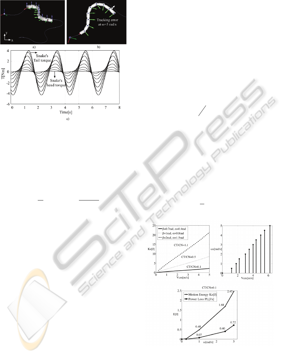
Figure 3: Snake-like robot simulation: a). Circular
serpenoid curve using
2.1=
γ
, b). Top view tracking
error due to inefficient friction and serpenoid parameters
tuning, c). Joint torques to move the snake forward.
Assuming the relation:
dm
=
m
⋅
L
−1
ds
(being
L
the
length of a body-i; see Figure 1), the friction torque
about the body-i CM is:
θθτ
3
2
0
2
,
mLC
dss
L
m
C
N
L
cdNcmr
−=−=
∫
(13)
Using Equations (11) and (13), the total friction
force vector denoted by Equation (7) is incorporated
into the dynamic’s EoM of the snake-like robot (see
Equation (6)).
Once the snake modelling is completed, Figure 3
depicts the 8-degree of freedom snake-like robot
(n=8) performing a circular serpenoid trajectory
profile:
α
= 0.5
rad
,
β
= 1.1
rad
,
ω
s
= 2.5
rad
/
s
.
Friction coefficients make the robot to generate
larger friction forces in the normal direction than in
the tangential direction of the motion. Considering
C
T
= 12
,
C
N
= 20
and the mass of each snake’s link
in
m
= 0.4
kg
. Despite the snake is capable of
propelling forward, a tracking error (caused by
external friction forces) appears when the snake is
speeding up. These preliminary results suggest us to
analyze how to relate energy consumption (input
power against speed), and how to tune friction
parameters as a function of that speed and serpenoid
curve terms. For this purpose, our goal in the next
section is to find how to change the serpenoid curve
parameters in Equation (2) to achieve the energy-
efficient locomotion based on the dynamic’s EoM in
Equation (6).
3 EFFICIENT SNAKE MOTION
Friction force represents a power loss. Part of the
input power generated by the snake’s actuators is
converted into kinetic energy
K
E
and the rest is lost
due to the friction.
The objective of this section is to find the
optimally efficient motion within the dynamics
framework of serpentine locomotion. More
precisely, our challenge is related to choosing the
parameters
α
,
β
,
ω
s
that make the average power
loss
P
L
in Equation (14) minimal while keeping a
prescribed average speed.
P
L
=
mV
i
T
−
C
N
m
L
2
3
0
0 0
.
c
θ
2
C
T
−
s
θ
2
C
N
s
θ
c
θ
C
T
−
C
N
( )
s
θ
c
θ
C
T
−
C
N
( )
s
θ
2
C
T
+
c
θ
2
C
N
V
i
(14)
The approach we used is to increase the speed of the
snake and verifying where is the saturation point that
preserves an efficient locomotion in terms of power
loss compared to the total energy of the system
described in Equation (15) as:
( )
i
T
i
n
i
E
JK
φφφ
∑
=
=
1
2
1
.
(15)
Figure 4: Energy and velocity relationship for different
average of serpenoid curve profiles
α
,
β
,
ω
s
for n=8.
The first set of tests consists on varying the
serpenoid curve parameters described in Equation
EFFICIENT LOCOMOTION ON NON-WHEELED SNAKE-LIKE ROBOTS
249
(2). Considering angular speeds from
ω
s
= [0...4]
,
we have analyzed the relationship between input
energy and speed. Results are shown in Figure 4.
Two preliminary important considerations can be
made. First of all, the relation to maintain between
friction coefficients as a function of the snake
morphology for n=8 (i.e. size, weight, mass
distribution), and the serpenoid curve profile (i.e.
undulation degree of the curve, speed, direction) is
about
C
T
/
C
N
= 0.1
. This friction ratio has been
found from taking the simulation-results average for
what choices of the serpenoid parameters
α
,
β
,
ω
s
the percentage of power loss is minimal. In this case,
at maximum serpentine speed angular propagation
of
ω
s
= 3
rad
/
s
, we achieved a maximum power loss
about 30%. Increasing the ratio of friction
coefficients under the same characteristics, the
energy consumption also increases and consequently
performance was compromised. Note that these
friction ratios strictly depend on the snake’s
dynamics and the terrain characteristics. For
experimental testing, we will have to explore and
test different kind of materials that achieve the
proper friction ratio dependent of different surfaces
of motion. Using this relation, the snake is capable
to move forward wasting the minimum energy and
achieving the required velocity; in other words, this
is the optimal relation between serpenoid curve
parameters, snake morphology, and friction forces.
In addition, also note in Figure 4 that using this
optimal relationship, the snake linear velocity
V
cm
and the serpenoid curve speed
ω
s
are roughly
proportional to each other.
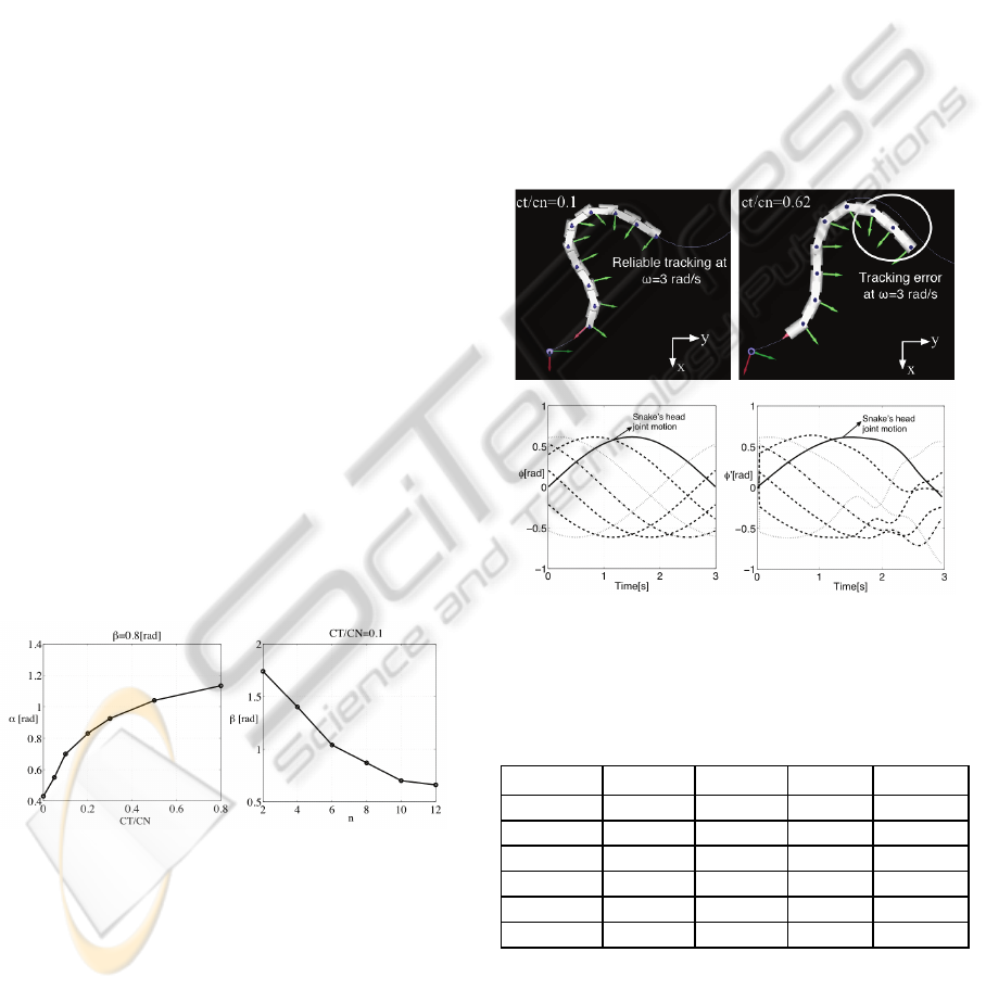
Figure 5: Serpenoid curve phase
β
and undulation degree
α
as a function of friction coefficients
C
T
/
C
N
and the
snake’s number of links n.
The tests performed in Figure 4, allowed us to find
the optimal energy relation between:
• Energy consumption
K
E
and
P
L
.
• Velocity
V
cm
and
ω
s
.
• Friction
C
T
/
C
N
and parameters
β
and
α
.
Nonetheless note from Equation 2 that
β
and
α
are
also strictly dependent on the snake configuration,
this means, the snake number of links: n.
Thus, we have carried out a second series of tests
varying the number of links (n) of the snake and
changing the terrain surface, i.e., changing ratios of
C
T
/
C
N
. From the results depicted in Figure 5, we
found that
α
is affected as a function of friction
modification, whereas
β
depends on the number of
links-n. Regarding the same simulation scenario in
Figure 3 (circular snake motion using
γ
= 1.2
o
), this
time we use optimal relationships to achieve energy-
efficient and reliable snake locomotion. The optimal
parameters configuration is:
α
= 0.7
rad
,
β
= 0.8
rad
,
n
= 8,
C
T
= 1,
C
N
= 10,
ω
s
= 3
rad
/
s
.
Figure 6 illustrates the simulation results for
open-loop tracking of the circular serpenoid path.
Figure 6: Cartesian (above) and Joint positions (below)
between efficient snake locomotion (left) against improper
parameters tuning (right), at snake speed of
ω
s
= 3
rad
/
s
.
Table 2: Efficiency of serpenoid locomotion for
C
T
/
C
N
= 0.1
.
Test-1 Test-2 Test-3 Test-4
ω
s
[rad/s] 0.25 1.04 2.5 3
%error
φ
0.59% 0.98% 1.15% 2.2%
K
E
[J] 0.022 0.48 1.68 2.45
P
L
[J/s] 9.2x10
-4
0.077 0.40 0.72
%
P
L
4.11%
5.75%
23.80%
29.38%
Efficiency 0.95 0.83 0.76 0.70
The simulation scenario shown in Figure 3 is now
compared to the efficient approach of serpentine
locomotion showed in Figure 6. The joint position
error
′
φ
(inefficient approach) is about 12.5%
against 2.2% for the efficient approach (
φ
). Table 2
ICINCO 2010 - 7th International Conference on Informatics in Control, Automation and Robotics
250
consigns several simulations on testing efficient
snake locomotion for different speed profiles.
4 CONCLUSIONS AND FUTURE
WORK
The dynamics framework for the modelling and
simulation of non-wheeled snake-like robots has
been presented. Bio-inspired kinematics locomotion
was efficiently integrated into our approach of
achieving efficient serpentine locomotion at high-
speeds. Simulation results depicted in Table II
showed that our first hypothesis was indeed correct.
Considering speeds up to 4 m/s we obtained efficient
motion (less than 30%) of power loss due to friction.
For speeds >4m/s, this efficiency decreases because
of the increase of the angular speed, which also
makes the friction force increases and subsequently
generating more power loss average that makes the
control effort too energetic. This speed boundary
was obtained from several simulations performed in
Figures 4 and 5. In conclusion, the key aspects in
regarding energy efficient serpentine locomotion are
basically synthesized as:
1).
α
is an increasing
function of
C
T
/
C
N
, thus, the snake robot should
undulate with larger amplitude when the friction
ratio is larger (i.e. the snake-like robot tends to slip
in the normal direction), 2).
ω
s
is basically a liner
function of the linear speed
V
cm
, and, 3).
β
is a
decreasing function of n.
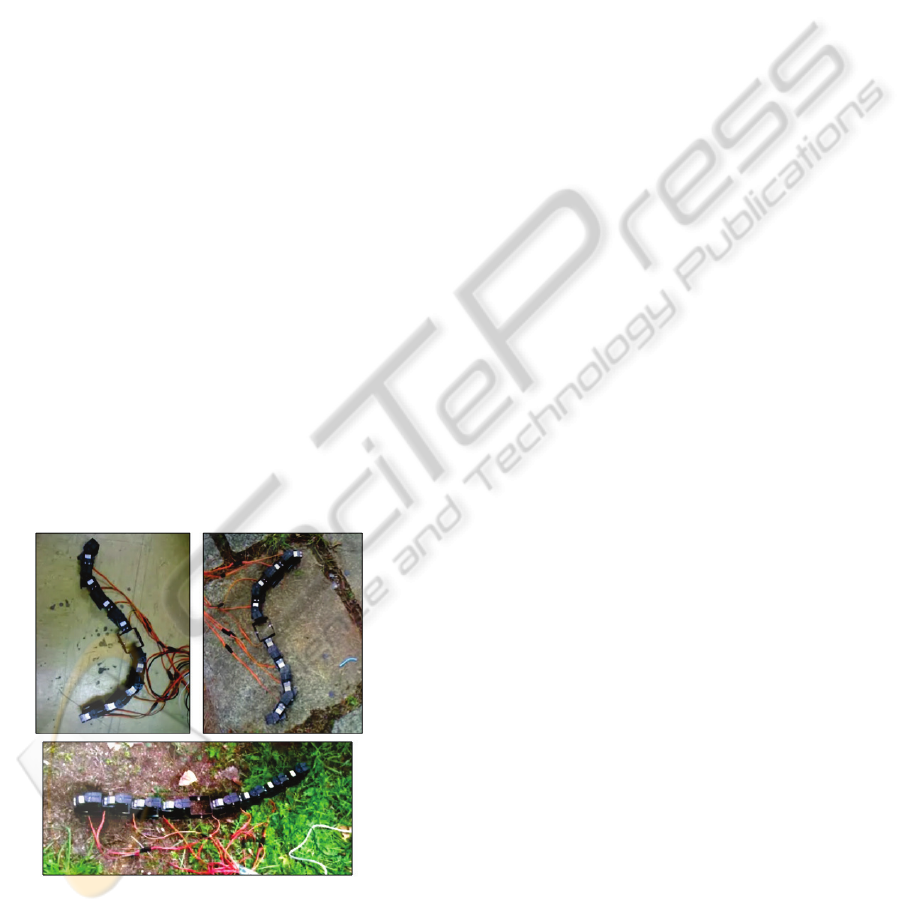
Figure 7: Locomotion testing experiments over different
friction terrains.
These relationships are useful for determining the
optimal control law for the snake robot. Upcoming
work is oriented towards the full implementation of
the hardware/software that allow the snake robot to
be fully controlled. Using a first prototype depicted
in Figure 7, our current work is focused on
researching which materials and shapes of the
snake’s skeleton generate the proper friction and
traction using our modeling approach.
ACKNOWLEDGEMENTS
This work is funded by the project ROBOCITY
2030 (S2009/DPI-1559).
REFERENCES
Chirikjian, G. S., and Burdick, J.W., 1990. An obstacle
avoidance algorithm for hyper-redundant ma-
nipulators. In IEEE International Conference on
Robotics and Automation, pag. 625–631, Cincinnati.
Dowling, K. J., 1997. Limbless Locomotion: Learning to
Crawl with a Snake Robot. PhD thesis, Carnegie
Melon University, Pittsburgh, USA.
Fu, K. S., Gonzalez, R.C., and Lee C.S.G., 1987.
Robotics: Control, Sensing, Vision, and Intelligence.
New York:McGraw-Hill.
Gray, J., and Lissmann, H., 1950. The kinetics of
locomotion of the grass-snake, J. Exp. Biol., vol. 26,
no. 4, pp. 354-367.
Hirose, S., 1993. Biologically inspired robots (snake-like
locomotor and manipulator). In Oxford University
Press.
Hirose, S., and Morishima, A., 1990. Design and control
of a mobile robot with an articulated body, Int. J.
Robot. Res., vol. 9, no. 2, pp. 99-114.
Kane, T., and Lecison, D., 2000. Locomotion of snakes:
A mechanical ‘explanation’, Int. J. Solids Struct., vol.
37, no. 41, pp. 5829–5837.
Kamegawa, T., Matsuno, F., and Chatterjee, R., 2002.
Proposition of Twisting Mode of Locomotion and GA
based Motion Planning for Transition of Locomotion
Modes of a 3-dimensional Snake-like Robot, Proc.
IEEE Int. Conf. on Robotics and Automation, pp. 1507
Ostrowski, J., 1995. The Mechanics of Control of
Undulatory Robotic Locomotion. PhD thesis,
California Institute of Technology.
Prautsch, P., and Mita, T., 1999. Control and Analysis of
the Gait of Snake Robots. Proceedings of the IEEE
International Conference on Control Applications,
Kohala Coast-Island of Hawaii, Hawaii, USA, pp.
502.
Transeth, A., and Pettersen, K.Y., 2006. Developments in
snake robot modeling and locomotion, in Proc. IEEE
Int. Conf. Control, Automation, Robotics and Vision,
pp. 1393–1400.
EFFICIENT LOCOMOTION ON NON-WHEELED SNAKE-LIKE ROBOTS
251
