
SURVEY OF ESTIMATE FUSION APPROACHES
Jiˇr´ı Ajgl and Miroslav
ˇ
Simandl
Department of Cybernetics, Faculty of Applied Sciences, University of West Bohemia in Pilsen
Univerzitn´ı 8, Plzeˇn, 306 14, Czech Republic
Keywords:
Dynamic systems, State estimation, Optimal estimation, Sensor fusion, Filtering problems.
Abstract:
The paper deals with fusion of state estimates of stochastic dynamic systems. The goal of the contribution
is to present main approaches to the estimate fusion which were developed during the last four decades. The
hierarchical and decentralised estimation are presented and main special cases are discussed. Namely the
following approaches, the distributed Kalman filter, maximum likelihood, channel filters, and the information
measure, are introduced. The approaches are illustrated in numerical examples.
1 INTRODUCTION
The classical estimation theory deals with estimating
the value of some attribute by using measured data.
(Simon, 2006) reviews the optimal state estimation
techniques for linear systems and their extension to
non-linear systems. However, there are other dimen-
sions of the estimation problem. The direction dis-
cussed here is the multisensor problem that assumes
the system state to be estimated by multiple estima-
tors. Each estimator uses different data sets and it can
communicate its estimate to the other estimators. The
question is how to combine multiple estimates to ob-
tain optimal results.
The key issues in the multisensor fusion are com-
munication and dependences. In practise, it is pos-
sible to communicate raw measurements among es-
timators. In such a case, each estimator can process
the measurements only and no estimate fusion is re-
quired. But in the case of the on-line state estimation
of dynamic systems the out-of-sequenceproblems oc-
curs. Updating the estimate by an old measurement is
complicated, see (Bar-Shalom, 2002) or (Challa et al.,
2003). Moreover, in general network of estimators,
the estimators must log a list of all measurements they
have processed or the measurement must be passed
with a list of estimators that have processed it. Oth-
erwise the multiple processing of the same data is in-
evitable.
If two estimators use measurements with depen-
dent errors, their estimates will be dependent. A non-
zero state noise causes dependence of the estimates
as well as the communication of the estimates with
the consequent fusion. The fused estimate and the es-
timates before fusion are obviously dependent. In a
rooted tree estimator network, some restarts of the es-
timators can be applied to solve the communication
dependence problem, see (Chong et al., 1999).
In the fusion point of view, the classical estima-
tion is named as centralised. A central estimator pro-
cesses raw measurements only. If the estimators are
organised in a rooted tree, the root is called a fusion
centre and the fusion is denoted as hierarchical or dis-
tributed. If there is not a fusion centre, the fusion is
decentralised. Only a local knowledge of the network
is usually assumed in these cases. The above men-
tioned approaches have been introduced in the litera-
ture by different ways during last decades. However,
a unique survey of the approaches is missing.
Therefore, the aim of the paper is to give a survey
of main results in estimate fusion and to show numer-
ical illustrations. Both hierarchical and decentralised
estimation are presented and discussed. In the hierar-
chical framework, namely the distributed Kalman fil-
ter and the fusion based on the maximum likelihood
estimation are considered. In the decentralised frame-
work, the stress is laid on the channel filters and the
information measure approach.
The paper is organised as follows. Section 2 de-
fines the fusion problem, section 3 and 4 discuss
the hierarchical and decentralised approaches, respec-
tively. A numerical example is given in section 5 and
finally section 6 summarises the fusion problems.
191
Ajgl J. and Šimandl M. (2010).
SURVEY OF ESTIMATE FUSION APPROACHES.
In Proceedings of the 7th International Conference on Informatics in Control, Automation and Robotics, pages 191-196
DOI: 10.5220/0002947201910196
Copyright
c
SciTePress

2 PROBLEM STATEMENT
Let the discrete-time stochastic system be described
by state transition and measurement conditional prob-
ability density functions
p(x
k+1
|x
k
), (1)
p(z
(1)
k
, z
(2)
k
, . . . , z
(N)
k
|x
k
). (2)
where z
( j)
k
, j = 1, . . . , N, are local measurements at
time k, k = 0, 1, . . . and the initial condition p(x
0
) is
known. Let the system be linear gaussian. In such
case, analytical solutions to estimation problems ex-
ist. The linear gaussian system can be described by
state and measurement equations
x
k+1
= Fx
k
+ Gw
k
, (3)
z
( j)
k
= H
( j)
x
k
+ v
( j)
k
, j = 1, . . . , N, (4)
where F ∈ R
n
x
×n
x
, H
( j)
∈ R
n
( j)
z
×n
x
, and G ∈ R
n
x
×n
w
are known matrices, x
k
∈ R
n
x
is the immeasurable
system state and z
( j)
k
∈ R
n
( j)
z
is the local measurement
coming from j-th sensor. The variables w
k
∈ R
n
w
and
v
( j)
k
∈ R
n
( j)
z
represent the state and measurement white
Gaussian noises with zero mean and with known co-
variance matrices Q, R
( j j)
, respectively. The pro-
cesses {v
( j)
k
} are independent of the process {w
k
} and
all of them are independent on the system initial state
described by the Gaussian pdf p(x
0
) = N (x
0
:
¯
x
0
, P
0
).
The measurement error processes {v
( j)
k
} can be gen-
erally mutually dependent, with cross-correlations
, R
(ij)
k
= E(v
(i)
k
v
( j)T
k
), but there are often assumed to
be independent, R
(ij)
k
= 0 for i 6= j.
Let each sensor have its estimator, i.e. there exist
N state estimates
ˆ
x
( j)
, j = 1, . . . , N, with correspond-
ing error covariance matrices P
( j)
. The estimators are
connected with some others by data link. The com-
munication network can be described by a directed
graph with nodes in each sensor and with edges rep-
resenting the oriented data links. It is assumed that
measurements coming from other sensor nodes can
not be processed directly, e.g. due to the unknown
measurement equation of the respective sensors, or
the communication of the measurements would be in-
effective. So it is assumed that only the estimates are
communicated. The goal of the fusion is to combine
local estimates.
3 HIERARCHICAL FUSION
In the hierarchical fusion, the local estimates are com-
municated to a fusion centre. The method are based
on the classical one-sensor estimation, which is de-
scribed in subsection 3.1. The distributed Kalman
filter extracts independent information from the esti-
mates and is discussed in subsection 3.2. In the max-
imum likelihood approach, the estimates are regarded
as dependent measurements. The respective fusion is
shown in subsection 3.3.
3.1 Optimal Centralised Estimate
In the case of one sensor system, there is no fusion
of estimates. The classical Kalman filter solution is
the exact Bayessian solution to the filtering problem
for a linear Gaussian system. You can see (Simon,
2006) for many numerical approximations to the ex-
act solution for non-linear systems. The Kalman filter
estimate is a standard against which other methods
can be compared. The filtering (measurement update)
equations
P
−1
k|k
ˆ
x
k|k
= P
−1
k|k−1
ˆ
x
k|k−1
+ H
T
k
R
−1
k
z
k
, (5)
P
−1
k|k
= P
−1
k|k−1
+ H
T
k
R
−1
k
H
k
, (6)
can be interpreted as a fusion of the predictive esti-
mate with the information based on the last measure-
ment only. The prediction (time update) equations
ˆ
x
k+1|k
= F
k
ˆ
x
k|k
, (7)
P
k+1|k
= F
k
P
k|k
F
T
k
+ Q
k
. (8)
correspond to the dynamics of the system. If more
explicit notation is required further in this article, the
general conditional pdf notation will be used. The
exact Bayessian solution is given by
p(x
k
|z
k
, Z
k−1
) ∝ p(z
k
|x
k
)p(x
k
|Z
k−1
) (9)
p(x
k+1
|Z
k
) =
Z
R
p(x
k+1
|x
k
)p(x
k
|Z
k
)dx
k
(10)
where ∝ means proportional to and Z
k
, {z
k
, Z
k−1
}
denotes the set of all measurements up to the time k.
The centralised estimator is a hypothetical estima-
tor which assumes that all measurements are immedi-
ately available to the estimator and that the correspon-
dent measurement equations are known at the centre.
The local measurement equations (4) can be merged
to one equation with
z
k
=
z
(1)
k
.
.
.
z
(N)
k
, H
k
=
H
(1)
k
.
.
.
H
(N)
k
, v
k
=
v
(1)
k
.
.
.
v
(N)
k
, (11)
R
k
= [R
(ij)
k
]
N
i, j=1
. The centralised Kalman filter is
given by (5)-(8) and (11).
ICINCO 2010 - 7th International Conference on Informatics in Control, Automation and Robotics
192

3.2 Distributed Kalman Filter
The distributed Kalman filter consists of N local
Kalman filters which send their estimates to one fu-
sion centre. It is also possible to distribute the local
filters recursively. The name hierarchical Kalman fil-
ter is also used. Note that the term decentralised is
misused in the literature to express that this filter is
not the centralised one.
The main assumption is the independence of the
local measurement errors,
R
(ij)
k
= 0, i 6= j. (12)
Then the pieces of information gained from the same
time measurements are independent and can be sim-
ply summed up. The fusion centre filtering equation
can be derived from (5), (6) with the use of (11) as
P
−1
k|k
ˆ
x
k|k
= P
−1
k|k−1
ˆ
x
k|k−1
+
+
N
∑
j=1
P
( j)
k|k
−1
ˆ
x
( j)
k|k
− P
( j)
k|k−1
−1
ˆ
x
( j)
k|k−1
, (13)
P
−1
k|k
= P
−1
k|k−1
+
N
∑
j=1
P
( j)
k|k
−1
− P
( j)
k|k−1
−1
, (14)
where indexes
( j)
denotes the local estimates. The fu-
sion centre predictive equations are identical to (7),
(8). It is possible to compute the predictive estimates
at each local estimator, but it requires to send predic-
tive estimate to the fusion centre. Instead of that, the
fusion centre predictive can be send to each local es-
timator where it replaces the local estimate
ˆ
x
( j)
k+1|k
←
ˆ
x
k+1|k
, P
( j)
k+1|k
← P
k+1|k
, (15)
j = 1, . . . , N. This feedback brings the globally opti-
mal estimate to each local estimator and the estima-
tion is expected to be better if the extension to non-
linear systems approximated by linearisation is con-
sidered.
The distributed Kalman filter for the system with
dependent noises is discussed in (Hashemipour et al.,
1988). (Berg and Durrant-Whyte, 1992) minimise the
communication by reducing the dimension of the es-
timated state at each local estimator and using intern-
odal transformations; there is no communication of
the state components that are not influenced by the
measurement.
The fusion centre filtering equations (13), (14) can
be written by the conditional densities as
p(x
k
|z
k
, Z
k−1
) ∝ p(x
k
|Z
k−1
)
N
∏
j=1
p(x
k
|z
( j)
k
, Z
k−1
)
p(x
k
|Z
k−1
)
,
(16)
where the feedback is given by
p(x
k
|z
( j)
k
, Z
k−1
) ← p(x
k
|Z
k
), (17)
j = 1, . . . , N, and is analogous to (15). Note that the
division by the predictive density p(x
k
|Z
k−1
) can not
be easily extended to general non-Gaussian densities.
3.3 Fusion by the Maximum Likelihood
This subsection discusses the fusion of dependent es-
timates at a fusion centre. The cornerstone idea is to
treat the local estimates as if they were measurements.
It arises from the identity, see (Li et al., 2003),
ˆ
x
( j)
k|k
= x
k
+ (
ˆ
x
( j)
k|k
− x
k
) = x
k
+ (−
˜
x
( j)
k|k
) (18)
where
˜
x
( j)
k|k
is the error of the estimate at the j-th es-
timator. The covariance matrices of these measure-
ments are the error covariance matrices P
( j j)
k|k
= P
( j)
k|k
.
Assuming the local estimates are obtained by Kalman
filters with Kalman gains K
( j)
k
= P
( j j)
k|k
H
( j)T
k
R
( j)
k
−1
,
the cross-covariancesP
(ij)
k|k
= E(
˜
x
(i)
k|k
˜
x
( j)T
k|k
) are given by
P
(ij)
k|k
= (I
n
x
− K
(i)
k
H
(i)
k
)P
(ij)
k|k−1
(I
n
x
− K
( j)
k
H
( j)
k
)
T
+
+K
(i)
k
R
(ij)
k
K
( j)T
k
, (19)
where I
n
x
is the identity matrix of the size n
x
, with the
initial condition P
(ij)
0|−1
= P
0
. The predictive covari-
ance P
(ij)
k|k−1
is computed by (8).
Then the fusion centre measurement equation is
given by
z
FC
k
= I
N
x
k
+ ξ
k
(20)
where cov(ξ
k
) = P
k
= [P
(ij)
k|k
]
N
i, j=1
and
z
FC
k
=
ˆ
x
(1)
k|k
.
.
.
ˆ
x
(N)
k|k
, I
N
=
I
n
x
.
.
.
I
n
x
, ξ
k
=
−
˜
x
(1)
k|k
.
.
.
−
˜
x
(N)
k|k
. (21)
Unfortunately, the process {ξ
k
} is correlated with x
k
and it is coloured, so it is not possible to use a Kalman
filter in the fusion centre. But the central estimate can
be obtained, see (Chang et al., 1997), by the maxi-
mum likelihood method
ˆ
x
k|k
= (I
T
N
P
−1
k
I
N
)
−1
I
T
N
P
−1
k
z
FC
k
, (22)
P
k|k
= (I
T
N
P
−1
k
I
N
)
−1
. (23)
Note that the above fusion requires to send the
Kalman filter gains K
( j)
k
, j = 1, . . . , N to the fusion
centre to compute the cross-correlations of the esti-
mates (19). The measurement matrices H
( j)
k
must be
known at or sent to the fusion centre also.
SURVEY OF ESTIMATE FUSION APPROACHES
193

4 DECENTRALISED FUSION
In the decentralised fusion, information is processed
localy. The channel filters enable to obtain a glob-
ally optimal solution in a tree network and they are
described in subsection 4.1. The information mea-
sure approach discussed in subsection 4.2 sacrifices
the Bayessian optimality for the the possibility to be
easily used in an arbitrary network.
4.1 Channel Filters
The principle of the channel filter approach, that was
introduced in (Grime and Durrant-Whyte, 1994), is
the same as that of the distributed Kalman filter in
fact. The new information is extracted and summed
up. The necessary condition is that there is one and
only one way of the information propagation, i.e. the
network structure is a tree. The density notation will
be used to explicitly denote the set of the measure-
ments that were exploited by each estimator.
The essential rule of the estimate fusion is
p(x
k
|Z
A
∪ Z
B
) =
p(x
k
|Z
A
)p(x
k
|Z
B
)
p(x
k
|Z
A
∩ Z
B
)
. (24)
The posterior probability density function of the state
conditioned on the union of two measurement sets is
equal to the product of the densities conditioned on
each measurement set divided by the density condi-
tioned on the intersection of the measurement sets.
The equation (24) is the core of the channel fil-
ters. It is assumed that all local measurement er-
rors are independent, (12). Thus, the measurement
density can be factorised, p(z
(1)
k
, z
(2)
k
, . . . , z
(N)
k
|x
k
) =
∏
N
j=1
p(z
( j)
k
|x
k
).
First, all local estimators filter their predictive es-
timates according to (9). Then the filtering estimates
are communicated to the neighbouring estimators.
The fusion is given by a repeated use of the fusion
rule (24) as
p(x
k
|Z
j
k
) = p(x
k
|z
( j)
k
, Z
j
k−1
)
∏
i∈N
j
p(x
k
|z
(i)
k
, Z
i
k−1
)
p(x
k
|Z
j
k−1
∩ Z
i
k−1
)
,
(25)
where Z
j
k
= (Z
j
k−1
∪ z
( j)
k
)
S
i∈N
j
(Z
i
k−1
∪ z
(i)
k
) is the set
of the measurements that were exploited by the j-th
estimator at the time k after the fusion with the in-
coming estimates p(x
k
|z
(i)
k
, Z
i
k−1
), N
j
is the set of the
neighbours of the j-th estimator that have sent their
estimates to it, and p(x
k
|Z
j
k−1
∩ Z
i
k−1
) is the estimate
of the channel filter ij. The fusion (25) uses the fact
that the measurement errors are independent and thus
(Z
i
k−1
∪ z
(i)
k
) ∩(Z
j
k−1
∪ z
( j)
k
) = Z
i
k−1
∩ Z
j
k−1
. (26)
The predictive estimates are computed according
to (10) and the channel filter estimate is given by
p(x
k
|Z
j
k
∩ Z
i
k
) =
p(x
k
|z
( j)
k
, Z
j
k−1
)p(x
k
|z
(i)
k
, Z
i
k−1
)
p(x
k
|Z
j
k−1
∩ Z
i
k−1
)
(27)
where the equations (24), (26) and the relation
(Z
i
k−1
∪ z
(i)
k
) ∪(Z
j
k−1
∪ z
( j)
k
) = Z
i
k
∩ Z
j
k
(28)
were used.
The local estimates equal to centralised estimates
with delayed measurements. The delays are given by
the length of the path between the respective sensors
decreased by one. Note that the division by the chan-
nel filter density in the equations (25) and (27) is eas-
ily tractable for Gaussian densities only.
4.2 Information Measure Approach
In general networks, the optimality cannot be reached
without inadequate effort. It can be impossible to de-
cide which measurements have been used to compute
the estimates. And even if this is possible, the com-
mon information in the denominator of (24) is too
complicated to find and to compute with. Multiple
processing of the same measurements, with the il-
lusion that the errors are independent, is inevitable.
Therefore to not underestimate the estimate error,
some bounds must be used.
The idea of the Covariance Intersection method,
see (Julier, 2009) for example, arises from the geo-
metrical interpretation of the estimates. The fused es-
timate {
ˆ
x, P} is required to be consistent, i.e. the error
covariance must not be underestimated, P − E[(x −
ˆ
x)(x −
ˆ
x)
T
]≥ 0, where x denotes the true state. As-
suming the local estimates {
ˆ
x
1
, P
1
}, {
ˆ
x
2
, P
2
} are con-
sistent, the convex combination of them
P
−1
ˆ
x = ωP
−1
1
ˆ
x
1
+ (1− ω)P
−1
2
ˆ
x
2
, (29)
P
−1
= ωP
−1
1
+ (1− ω)P
−1
2
, (30)
where ω ∈ [0, 1], leads to consistent estimate {
ˆ
x, P}
for arbitrary cross-covariance P
12
= E[(x −
ˆ
x
1
)(x −
ˆ
x
2
)
T
], i.e. for arbitrary common information.
The weight ω can be chosen in order to minimise
various criteria. The usual criterion is the determinant
of the fused error covariance matrix,
ω
∗
= argmin
ω∈[0,1]
(detP), (31)
but the trace tr(P) is also used. The optimal weight ω
∗
can be approximated by the use of fast algorithms, see
(Fr¨anken and H¨upper, 2005). Special covariance con-
sistency methods can be found in (Uhlmann, 2003).
ICINCO 2010 - 7th International Conference on Informatics in Control, Automation and Robotics
194
(Hurley, 2002) generalise the Covariance Intersec-
tion method to the combination of probability density
functions. The geometrical combination
p
ω
(x) =
p
ω
1
(x)p
1−ω
2
(x)
R
R
p
ω
1
(x)p
1−ω
2
(x)dx
(32)
is used and the criterion of entropy, i.e. the Shannon
information, of the fused density
H (p
ω
) = −
Z
R
p
ω
(x)ln p
ω
(x)dx, (33)
that corresponds to the determinant criterion of the
fused estimate of Gaussian density, can be applied.
Other proposed criterion is the Chernoff information
C (p
1
, p
2
) = − min
0≤ω≤1
ln
R
R
p
ω
1
p
1−ω
2
(x)dx
. The
optimal density is equally distant from the local
densities in the Kullback-Leibler divergence sense,
D (p
ω
∗
k p
1
) = D (p
ω
∗
k p
2
), where the Kullback-
Leibler divergence is defined as D (p
1
k p
2
) =
R
R
p
1
(x)ln
p
1
(x)
p
2
(x)
dx. (Julier, 2006) studies the Cher-
noff fusion approximation for Gausian-mixture mod-
els, (Farrell and Ganesh, 2009) and (Wang and Li,
2009) consider fast convex combination methods.
5 NUMERICAL ILLUSTRATION
In this section, the fusion approaches will be illus-
trated by a numerical example. Let the system (3), (4)
with three sensors be t-invariant and given by
F = I
2
, G = I
2
, Q =
1.44 −1.2
−1.2 1
, (34)
H
(1)
=
1 0
, R
(11)
= 1,
H
(2)
=
1 −1
, R
(22)
= 2,
H
(3)
=
0 1
, R
(33)
= 1,
(35)
where the measurement errors are independent,
R
(12)
= R
(13)
= R
(23)
= 0, and the initial condition
is given by p(x
0
) = N ([0, 0]
T
, I
2
).
The used hierarchical and decentralised networks
are shown on the Fig. 1, the numbers denote the re-
spective estimators. The data links 1 ↔ 2 and 2 ↔ 3
are considered in the decentralised network.
Figure 1: Hierarchical (left) and decentralised network
(right), FC = fusion centre.
The centralised fusion (11), will be compared with
the maximum likelihood (21), (22), (23), distributed
Kalman filter (13)-(15), channel filters (25), (27) and
the information measure approaches (29)-(31). The
1-σ bounds, i.e. the multidimensional parallels of the
standard deviation, will show the uncertainty of the
fused estimates. The bounds will be centred to zero to
allow a better graphical comparison and are given by
{x : x
T
P
−1
x = 1}, where P is the estimate covariance
and the x = [x
1
, x
2
]
T
.
All estimators, including the fusion centre of the
distributed Kalman filter and the channel filters, have
the same initial condition p(x
0
). The system is sim-
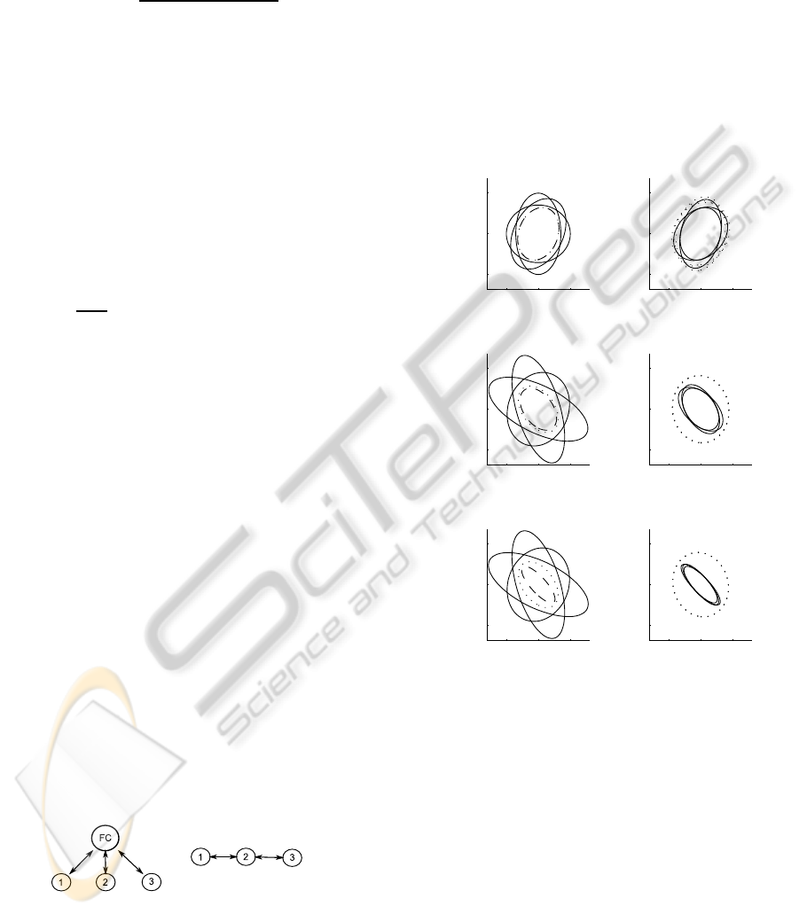
ulated and the 1-σ bounds at the times k = 1, k = 5,
and k = 20 are shown in the Fig. 2 for the hierarchical
and decentralised estimators.
−1 0 1
−1
0
1
x
1,1
x
2,1
−1 0 1
−1
0
1
x
1,1
x
2,1
−1 0 1
−1
0
1
x
1,5
x
2,5
−1 0 1
−1
0
1
x
1,5
x
2,5
−1 0 1
−1
0
1
x
1,20
x
2,20
−1 0 1
−1
0
1
x
1,20
x
2,20
Figure 2: A comparison of the 1-σ bounds of the hierarchi-
cal and decentralised estimates at times k = 1, 5, 20.
The left half of the Fig. 2 shows the optimal
centralised estimator (dashed line), the distributed
Kalman filter (with the same estimate - dashed line),
local Kalman filters (solid lines), and the fusion by the
maximum likelihood at the fusion centre (dotted line).
At the time k = 1 (top), the maximum likelihood es-
timate and the centralised estimate have equal covari-
ances, the lines seem to be dash-dotted. At the times
k = 5 and k = 20 (middle and bottom), the influence
of not incorporating the prior information is evident,
the covariance of the maximum likelihood estimate is
greater than that of the centralised estimate. The local
filters are the least accurate.
SURVEY OF ESTIMATE FUSION APPROACHES
195

The right half of the Fig. 2 shows the local esti-
mates with the channel filter fusion (solid lines) and
the Covariance Intersection fusion (dotted lines). The
estimate of the estimator 2 with the channel filter fu-
sion is equal to the centralised estimate in this case.
The one-step delay of the measurement exploitation
in the estimators 1 (which measures x
1
) and 3 (which
measures x
2
) is visible, there is greater uncertainty in
the x
2
and x
1
axis, respectively. The the local esti-
mates which use the Covariance Intersection get close
to each other after a few steps. In this example, the es-
timates 2 and 1 are fused first and the result is fused
with the estimate 3. The estimates overestimate the
error covariance, but at least they are not worse than
the estimates that use local measurements only with-
out any fusion (compare with the solid lines on the
left half of the figure). The information measure ap-
proaches are useful for more complex networks.
6 SUMMARY
Main approaches to the state estimate fusion for the
linear stochastic systems were introduced. The princi-
ples and algorithms of hierarchical and decentralised
fusion were presented and discussed. Contrary to the
standard estimation problem, which is based on using
all measurements simultaneously, the estimate fusion
allows to respect an alternative technical specification
concerning the measurement location and to prefer lo-
cal information processing. The hierarchical fusion
is more suitable for systems with a small number of
sensors. In the case of general network with many
sensors, the decentralised fusion based on informa-
tion measures should be preferred due to its simplicity
and modest assumptions.
ACKNOWLEDGEMENTS
This work was supported by the Ministry of Educa-
tion, Youth and Sports of the Czech Republic, project
no. 1M0572, and by the Czech Science Foundation,
project no. 102/08/0442.
REFERENCES
Bar-Shalom, Y. (2002). Update with out-of-sequence mea-
surements in tracking: Exact solution. IEEE Transac-
tions on AES, 38(3):760–778.
Berg, T. M. and Durrant-Whyte, H. F. (1992). Distributed
and decentralized estimation. In SICICI ’92 proceed-
ings, volume 2, pages 1118–1123.
Challa, S., Evans, R. J., and Wang, X. (2003). A
bayesian solution and its approximations to out-of-
sequence measurement problems. Information Fu-
sion, 4(3):185–199.
Chang, K.-C., Sahat, R. K., and Bar-Shalom, Y. (1997). On
optimal track-to-track fusion. IEEE Transactions on
AES, 33(4):1271–1276.
Chong, C.-Y., Mori, S., Chang, K.-C., and H., B. W. (1999).
Architectures and algorithms for track association and
fusion. In Proceedings of the 2nd International Conf.
on Information Fusion.
Farrell, W. J. and Ganesh, C. (2009). Generalized chernoff
fusion approximation for practical distributed data fu-
sion. In Proceedings of the 12th International Conf.
on Information Fusion.
Fr¨anken, D. and H¨upper, A. (2005). Improved fast covari-
ance intersection for distributed data fusion. In Proc.
of the 8th Int. Conf. on Inf. Fusion.
Grime, S. and Durrant-Whyte, H. F. (1994). Data fusion in
decentralized sensor networks. Control Engineering
Practice, 3(5):849–863.
Hashemipour, H. R., Roy, S., and Laub, A. J. (1988).
Decentralized structures for parallel kalman filtering.
IEEE Transactions on AuC, 33(1):88–94.
Hurley, M. B. (2002). An information theoretic justifica-
tion for covariance intersection and its generalization.
In Proceedings of the 5th International Conference on
Information Fusion.
Julier, S. J. (2006). An empirical study into the use of cher-
noff information for robust, distributed fusion of gaus-
sian mixture models. In Proceedings of the 9th Int.
Conf. on Information Fusion.
Julier, S. J. (2009). Estimating and exploiting the degree of
independent information in distributed data fusion. In
Proceedings of the 12th International Conference on
Information Fusion.
Li, X.-R., Zhu, Y., Wang, J., and Han, C. (2003). Opti-
mal linear estimation fusion—part i: Unified fusion
rules. IEEE Transactions on Information Theory,
49(9):2192–2208.
Simon, D. (2006). Optimal State Estimation. Wiley.
Uhlmann, J. K. (2003). Covariance consistency methods
for fault-tolerant distributed data fusion. Information
Fusion, 4(3):201–215.
Wang, Y. and Li, X.-R. (2009). A fast and fault-tolerant
convex combination fusion algorithm under unknown
cross-correlation. In Proceedings of the 12th Int. Conf.
on Information Fusion.
ICINCO 2010 - 7th International Conference on Informatics in Control, Automation and Robotics
196
