
REINFORCEMENT LEARNING FOR ROBOT CONTROL
USING PROBABILITY DENSITY ESTIMATIONS
Alejandro Agostini and Enric Celaya
Institut de rob`otica i Inform`atica Industrial, (CSIC-UPC), Barcelona, Spain
Keywords:
Machine Learning in control applications, Reinforcement learning.
Abstract:
The successful application of Reinforcement Learning (RL) techniques to robot control is limited by the fact
that, in most robotic tasks, the state and action spaces are continuous, multidimensional, and in essence, too
large for conventional RL algorithms to work. The well known curse of dimensionality makes infeasible using
a tabular representation of the value function, which is the classical approach that provides convergence guar-
antees. When a function approximation technique is used to generalize among similar states, the convergence
of the algorithm is compromised, since updates unavoidably affect an extended region of the domain, that is,
some situations are modified in a way that has not been really experienced, and the update may degrade the ap-
proximation. We propose a RL algorithm that uses a probability density estimation in the joint space of states,
actions and Q-values as a means of function approximation. This allows us to devise an updating approach
that, taking into account the local sampling density, avoids an excessive modification of the approximation far
from the observed sample.
1 INTRODUCTION
Any robotic application requires a precise control of
the robot effectors. In many situations, the design of
the control system and the necessary tuning of its pa-
rameters becomes a hard task, and there is a great in-
terest in providing the robot with the ability to learn
by itself how to control its effectors through experi-
ence. The most usual approach to achieve this is Re-
inforcement Learning (RL) (Sutton and Barto, 1998),
in which the robot must find an optimal action policy
by trial and error using a signal, called reinforcement,
that tells how good was the result obtained after each
executed action.
Reinforcement Learning algorithms, like value it-
eration or policy iteration, are known to converge in
the case of finite state-action spaces, where a tabu-
lar representation of the value function or the utility
function Q can be used. However, in a typical robot
control problem, the state and action spaces are con-
tinuous or too large, so that it is necessary to use
some form of function approximation. In this case
convergence is no longer granted in general, and this
is attributed to the fact that the update on the func-
tion approximation that takes place after each expe-
rience is not local to the precise observed point in
the state-action space, but influences the values in
other regions, possibly undoing the learning done so
far (Riedmiller, 2005a). This problem is magnified
when the sampling of the domain is too biased, caus-
ing some regions to be updated much more oftenly
than others.
Recently, much work has been done in RL with
function approximation. For example, (Ernst et al.,
2005) proposed the fitted Q Iteration algorithm, based
on previous work of (Ormoneit and Sen, 2002)
on kernel-based RL, and using randomized trees
for function approximation. Similarly, (Riedmiller,
2005a) proposed the Neural Fitted Q Iteration (NFQ)
algorithm, which uses a multi-layer perceptron for
function representation. In a different approach, (Ras-
mussen and Kuss, 2004) used Gaussian Processes
(GP) to model the system dynamics, and a further GP
to represent the Value function. The same approach
is followed by (Rottmann and Burgard, 2009), while
(Engel et al., 2005) used a GP to directly represent
the Q-function in a model-free setting. All these algo-
rithms fall into the class of the so-called fitted value
iteration algorithms (Gordon, 1995), which, in order
to approximate the desired function, take a finite num-
ber of training samples and try to fit the function to
them in a batch, iterative process. The usual approach
160
Agostini A. and Celaya E. (2010).
REINFORCEMENT LEARNING FOR ROBOT CONTROL USING PROBABILITY DENSITY ESTIMATIONS.
In Proceedings of the 7th International Conference on Informatics in Control, Automation and Robotics, pages 160-168
DOI: 10.5220/0002949601600168
Copyright
c
SciTePress

to obtain the training samples, when the knowledge
of the system dynamics is available, consists in sam-
pling uniformly all the state-action space to build a
training set that covers all possible situations suffi-
ciently well. Clearly, this procedure is not possible
when dealing with a real system with unknown dy-
namics, in what case samples can only be observed
while interacting with the real system. In the sim-
plest cases, it is possible to roughly cover the whole
state space by chaining a number of random actions,
as in (Ernst et al., 2005). However, when the prob-
lem grows in complexity, the probability of executing
a random sequence that drives the system to the inter-
esting regions of the workspace may be too low to be
achieved in practical time. In such cases it is neces-
sary to exploit the knowledge already obtained with
previous interactions (Riedmiller, 2005a; Ernst et al.,
2005).
It has to be noted that the need of exploiting what
has been learned so far introduces a tendency to ex-
perience the most promising states much more of-
tenly than others, and this systematically produces a
very biased sampling that aggravates the perturbing
effect caused by non-local updating pointed out be-
fore. In (Riedmiller, 2005a), this problem is avoided
by assuring that all datapoints are used for update the
same number of times. This is made possible by re-
membering a dense enough set of transitions and per-
forming full updates in batch mode. In fact this is a
common trait of all fitted value iteration algorithms.
From a computational point of view, this approach
is very computationally intensive, since all datapoints
are used a large number of times until convergence is
reached. A more efficient approach would result if,
instead of retraining with old data in batch, an incre-
mental updating could be achieved in which the per-
turbing effect of new samples on old estimations was
attenuated.
In the present work, we address the problem of the
biased sampling with incremental updating. In our
approach, we take into account how often each region
of the domain has been visited, updating more locally
those regions that are more densely sampled. To do
this, we need an estimation of the sampling density,
for what we use a Gaussian Mixture Model (GMM)
representing a probability density of samples in the
joint space of states, actions, and Q-values. At the
same time, this density estimation can be used as a
means of function approximation for the Q-function.
Density estimations are receiving increasing interest
in the field of machine learning (Bishop, 2006), since
they keep all the information contained in the data,
that is, they provide estimations not only for the ex-
pected function value, but also for its uncertainty.
Despite density estimations are more demanding
than simple function approximation (due to the fact
that they embody more information), their use for
function approximation has been advocated by differ-
ent authors (Figueiredo, 2000; Ghahramani and Jor-
dan, 1994), noting that simple and well understood
tools like the Expectation-Maximization (EM) algo-
rithm (Dempster et al., 1977) can be used to obtain
accurate estimations of the density function.
The rest of the paper is organized as follows: Sec-
tion 2 briefly resumes the basics of RL. Section 3 in-
troduces the concepts of GMM for multivariate den-
sity estimation, and the EM algorithm in its batch ver-
sion. In Section 4 we define the on-line EM algorithm
for the GMM. In Section 5, we present our approach
to deal with biased sampling. In Section 6 we develop
our RL algorithm using density estimation of the Q-
value function, involving action evaluation and action
selection. Section 7 describes the test control applica-
tion to show the feasibility of the approach. We con-
clude in Section 8 with a discussion of the proposed
approach.
2 THE REINFORCEMENT
LEARNING PARADIGM
In the RL paradigm, an agent must improve its per-
formance by selecting actions that maximize the ac-
cumulation of rewards provided by the environment
(Sutton and Barto, 1998). At each time step, the agent
observes the current state s
t
and chooses an action a
t
according to its policy a = π(s). The environment
changes to state s
t+1
in response to this action, and
produces an instantaneous reward r(s
t
,a
t
). The agent
must experiment by interacting with the environment
in order to find the optimal action policy from the out-
come of its past experiences. One of the most pop-
ular algorithms used in RL is Q-Learning (Watkins
and Dayan, 1992), which uses an action-value func-
tion Q(s,a) to estimate the maximum expected future
cumulative reward that can be obtained by executing
action a in situation s and acting optimally thereafter.
Q-learning uses a sampled version of the Bellman op-
timality equations (Bellman and Dreyfus, 1962) to es-
timate instantaneous q values,
q(s
t
,a
t
) = r(s
t
,a
t
) + γmax
a
Q(s
t+1
,a) (1)
where max
a
Q(s
t+1
,a) is the estimated maximum cu-
mulative reward corresponding to the next observed
situation s
t+1
, and γ is a discount factor, with values in
[0,1] that regulates the importance of future rewards
with respect to immediate ones. At a given stage of
REINFORCEMENT LEARNING FOR ROBOT CONTROL USING PROBABILITY DENSITY ESTIMATIONS
161

the learning, the temporary policy can be derived from
the estimated Q-function as,
π(s) = argmax
a
Q(s,a) (2)
In actor/critic architectures, a policy function
(called the actor) is learned and explicitly stored, so
that actions are directly decided by the actor and do
not need to be computed from the maximization in
(2). Despite this computational advantage, the learn-
ing of an actor may slow down convergence, since
then the learning of the Q-function must be done on-
policy instead of off-policy, and both functions, actor
and critic, must adapt to each other to reach conver-
gence. In our implementation we avoid the use of an
actor, and thus we must face the problem of maximiz-
ing the Q(s,a) function in (2).
The basic formulation of Q-learning assumes dis-
crete state-action spaces and the Q-function is stored
in a tabular representation. For continuous domains
a function approximation is required to represent the
Q-function and generalize among similar situations.
In next sections we present our proposal for function
approximation using density estimations.
3 DENSITY ESTIMATION WITH
A GAUSSIAN MIXTURE
MODEL
A Gaussian Mixture Model (Bishop, 2006) is a
weighted sum of multivariate Gaussian probability
density functions, and is used to represent general
probability density distributions in multidimensional
spaces. It is assumed that the samples of the distri-
bution to be represented have been generated through
the following process: first, one Gaussian is randomly
selected with a priori given probabilities, and then,
a sample is randomly generated with the probabil-
ity distribution of the selected Gaussian. According
to this, the probability density function of generating
sample x is:
p(x;Θ) =
K
∑
i=1
α
i
G(x;µ
i
,Σ
i
) (3)
where K is the number of Gaussians of the mix-
ture; α
i
, usually denoted as the mixing parameter, is
the prior probability, P(i), of Gaussian i to generate
a sample; G(x;µ
i
,Σ
i
) is a multidimensional normal
Gaussian function with mean vector µ
i
and covariance
matrix Σ
i
; and Θ = {{α
1
,µ
1
,Σ
1
},...,{α
K
,µ
K
,Σ
K
}} is
the whole set of parameters of the mixture. By al-
lowing the adaption of the number K of Gaussians
in the mixture, any smooth density distribution can
be approximated arbitrarily close (Figueiredo, 2000).
The parameters of the model can be estimated using a
maximum-likelihood estimator (MLE). Given a set of
samples X = {x
t
;t = 1,... ,N}, the likelihood func-
tion is given by
L[X;Θ] =
N
∏
t=1
p(x
t
;Θ). (4)
The maximum-likelihood estimation of the model pa-
rameters is the Θ that maximizes the likelihood (4)
for the data set X. Direct computation of the MLE
requires complete information about which mixture
component generated which instance. Since this in-
formation is missing, the EM algorithm, described in
the next section, is often used.
3.1 The Expectation-maximization
Algorithm
The Expectation-Maximization (EM) algorithm
(Dempster et al., 1977) is a general tool that permits
to estimate the parameters that maximize the likeli-
hood function (4) for a board class of problems when
there are some missing data. The EM method first
produces an estimation of the expected values of the
missing data using initial values of the parameters to
be estimated (E step), and then computes the MLE
of the parameters given the expected values of the
missing data (M step). This process is repeated
iteratively until a convergence criterion is fulfilled.
In this section we briefly describe how EM is ap-
plied to the specific case of a GMM. The process
starts with an initialization of the mean vectors and
covariancematrices of the Gaussians. The E step con-
sists in obtaining the probability P(i|x
t
) for each com-
ponent i of generating instance x
t
, that we denote by
w
t,i
,
w
t,i
= P(i|x
t
) =
P(i)p(x
t
|i)
K
∑
j=1
P( j)p(x
t
| j)
=
α
i
G(x
t
;µ
i
,Σ
i
)
K
∑
j=1
α
j
G(x
t
;µ
j
,Σ
j
)
(5)
where t = 1,..,N and i = 1, ..,K. The maximiza-
tion step consists in computing the MLE using the
estimated w
t,i
. It can be shown (Duda et al., 2001)
that, for the case of a GMM, the mixing parameters,
means, and covariances are given by
α
i
=
1
N
N
∑
t=1
w
t,i
(6)
µ
i
=
N
∑
t=1
w
t,i
x
t
N
∑
t=1
w
t,i
(7)
ICINCO 2010 - 7th International Conference on Informatics in Control, Automation and Robotics
162

Σ
i
=
N
∑
t=1
w
t,i
(x
t
− µ
i
)(x
t
− µ
i
)
T
N
∑
t=1
w
t,i
(8)
4 ON-LINE EM
Estimating a probability density distribution by
means of the EM algorithm involves the iteration of
E and M steps on the complete set of available data,
that is, the mode of operation of EM is in batch. How-
ever, in Q-learning, sample data are not all available
at once: they arrive sequentially and must be used
online to improve the policy that will allow an effi-
cient exploration-exploitation strategy. This prevents
the use of the batch EM algorithm, and requires an
on-line, incremental version of it. Several incremen-
tal EM algorithms have been proposed for the Gaus-
sian Mixture Model applied to clustering or classifica-
tion of stationary data (Song and Wang, 2005; Arand-
jelovic and Cipolla, 2005).
The approach proposed in (Song and Wang, 2005)
in not strictly an on-line EM algorithm. It applies
the conventional batch EM algorithm onto separate
data streams corresponding to successive episodes.
For each new stream, a new GMM model is trained
in batch mode and then merged with the previous
model. The number of components for each new
GMM is defined using the Bayesian Information Cri-
terion, and the merging process involves similarity
comparisons between Gaussians. This method in-
volves many computationally expensive processes at
each episode and tends to generate more components
than actually needed. The applicability of this method
to RL seems limited, not only for its computational
cost, but also because, due to the non-stationarity
of the Q-estimation, old data should not be taken as
equally valid during all the process.
The work of (Arandjelovic and Cipolla, 2005)
performs incremental updating of the density model
using no historical data and assuming that consecu-
tive data vary smoothly. The method maintains two
GMMs: the current GMM estimation, and a previous
GMM of the same complexity after which no model
updating (i.e. no change in the number of Gaussians)
has been done. By comparing the current GMM with
the historical one, it is determined if new Gaussians
are generated or if some Gaussians are merged to-
gether. Two observed shortcomings of the algorithm
are that the system fails when new data is well ex-
plained by the historical GMM, and when consecutive
data violate the condition of smooth variation.
In (Sato and Ishii, 2000), an on-line EM algorithm
is presented for the Normalized Gaussian Network
(NGnet), a model closely related to the GMM. This
algorithm is based on the works of (Nowlan, 1991;
Neal and Hinton, 1998). In (Nowlan, 1991) a method
for the incremental adaptation of the model param-
eters using a forgetting factor and cumulative statis-
tics is proposed, while in (Neal and Hinton, 1998)
the method in (Nowlan, 1991) is evaluated and con-
trasted with an incremental version which performs
steps of EM over a fixed set of samples in an incre-
mental way. The method proposed in (Sato and Ishii,
2000) uses foundations of both works to elaborate an
on-line learning algorithm to train a NGnet for regres-
sion, where weighted averages of the model parame-
ters are calculated using a learning rate that implic-
itly incorporates a forgetting factor to deal with non-
stationarities. Inspired by this work, we developed
an on-line EM algorithm for the GMM. Our approach
uses cumulative statistics whose updating involves a
forgetting factor explicitly.
4.1 On-line EM for the GMM
In the on-line EM approach, an E step and an M step
are performed after the observation of each individual
sample. The E step does not differ from the batch ver-
sion (equation (5)), except that it is only computed for
the new sample. For the M step, the parameters of all
mixture components are updated with the new sam-
ple. For this, we define the following time-discounted
weighted sums
W
t,i
= [[1]]
t,i
(9)
X
t,i
= [[x]]
t,i
(10)
(XX)
t,i
=
(x− µ
i
)(x− µ
i
)
T
t,i
(11)
where we use the notation:
[[ f]]
t,i
=
t
∑
τ=1
t
∏
s=τ+1
λ
s
!
f
τ,i
w
τ,i
(12)
where λ
t
, which ranges in [0,1], is a time dependent
discount factor introduced for forgetting the effect of
old, possibly outdated values. Observe that for low
values of λ
t
, the influence of old data decreases pro-
gressively, so that they are forgotten along time. This
forgetting effect of old data is attenuated when λ
t
ap-
proaches 1: in this case, old and new data have the
same influence in the sum. As learning proceeds and
data values become more stable, forgetting them is no
more required and λ
t
can be made to progressively
approach 1 to reach convergence.
The discounted sum W
t,i
can be interpreted as the
accumulated number of samples (composed of frac-
tions w
t,i
) attributed to unit i along time, with forget-
ting. Similarly, X
t,i
corresponds to the accumulated
REINFORCEMENT LEARNING FOR ROBOT CONTROL USING PROBABILITY DENSITY ESTIMATIONS
163

sum with forgetting of sample vectors x attributed to
unit i, which is used to derive the mean vector µ
i
. In
the same way, (XX)
t,i
accumulates the matrices of co-
variances of the vectors x attributed to unit i, which
are used to calculate the covariance matrix Σ
i
.
From (12), we obtain the recursive formula:
[[ f]]
t,i
= λ
t
[[ f]]
t−1,i
+ f
t,i
w
t,i
(13)
When a new sample x
t
arrives, all the accumulators
are updated with the incremental formula (13), and
new estimators for the GMM parameters are obtained
as:
α
t,i
=
W
t,i
K
∑
j=1
W
t,i
(14)
µ
t,i
=
X
t,i
W
t,i
(15)
Σ
t,i
=
(XX)
t,i
W
t,i
. (16)
The approximation capabilities of a GMM depend
on the number K of Gaussians of the mixture. Since
we can not determine the most appropriate number
beforehand, the number of Gaussians can be incre-
mented on-line. We delay the explanation of the pro-
cess for unit generation until Section 6.2.
5 DEALING WITH BIASED
SAMPLING
In the incremental formula (13), the factor λ
t
is used
to progressively replace (forget) old data by new ar-
rived ones in a smooth way. This is the desired ef-
fect when data are presented in a statistically unbi-
ased way, so that all past entries are equally forgotten
at the arrival of each new sample. However, in RL,
data are not uniformly distributed on the state-action
space, but are obtained along the trajectories followed
by the agent, and are particularly biased toward the
good-valued regions due to the need for exploitation.
That is, convergenceregions are more frequently sam-
pled, causing their densities to increase, but this is at
the expense of lowering densities and forgetting data
in other regions. This is undesirable since, statistics
in regions with low Q values, and hence sparsely sam-
pled, will get their data lost. This can be seen by set-
ting w
t,i
= 0 in equation (13), what yields:
[[ f]]
t,i
= λ
t
[[ f]]
t−1,i
, (17)
showingthat the accumulators of units that are seldom
activated will decay to 0. To avoid this we modify the
updating formula (13) in this way,
[[ f]]
t,i
= λ
w
t,i
t
[[ f]]
t−1,i
+ f
t,i
w
t,i
. (18)
In this updating formula, the power w
t,i
prevents
undesired changes in the parameters of the Gaussians
which are not responsible of generating the observed
values. Thus, if we make w
t,i
= 0 in (18), what we get
is:
[[ f]]
t,i
= [[ f]]
t−1,i
, (19)
so that the values of the statistics of the inactive units
remain unchanged. On the other hand, in the limit
case of w
t,i
= 1, corresponding to a full activation of
unit i, the effect of the new updating formula is the
same as before:
[[ f]]
t,i
= λ
t
[[ f]]
t−1,i
+ f
t,i
(20)
Therefore, we will adopt the updating formula (18)
that keeps better track of less explored regions.
6 Q-LEARNING WITH A GMM
In the case of Q-Learning, samples are of the form
x
t
= (s
t
,a
t
,q(s
t
,a
t
)), consisting of the visited state
s
t
, the executed action a
t
, and the estimated value of
q(s
t
,a
t
) as given by eq. (1). To obtain this estimation
we need to evaluate max
a
Q(s
t+1
,a), where Q(s,a) is
defined as the expected value of q given s and a for the
joint probability distribution provided by the GMM:
p(s,a,q) =
K
∑
i=1
α
i
G(s,a,q;µ
i
,Σ
i
), (21)
Q(s,a) = E [q|s,a] = µ(q|s,a) (22)
To compute this, we must first obtain the distribution
p(q|s,a). Decomposing the covariances Σ
i
and means
µ
i
in the following way:
µ
i
=
µ
(s,a)
i
µ
q
i
(23)
Σ
i
=
Σ
(s,a)(s,a)
i
Σ
(s,a)q
i
Σ
q(s,a)
i
Σ
qq
i
!
, (24)
the probability distribution of q, for the given state s
and a tentative action a, can then be expressed as:
p(q|s,a) =
K
∑
i=1
β
i
(s,a)G (q;µ
i
(q|s,a),σ
i
(q)) (25)
where,
µ
i
(q|s,a) = µ
q
i
+Σ
q(s,a)
i
Σ
(s,a)(s,a)
i
−1
(s,a) − µ
(s,a)
i
(26)
σ
2
i
(q) = Σ
qq
i
− Σ
q(s,a)
i
Σ
(s,a)(s,a)
i
−1
Σ
(s,a)q
i
(27)
ICINCO 2010 - 7th International Conference on Informatics in Control, Automation and Robotics
164

β
i
(s,a) =
α
i
G(s,a;µ
(s,a)
i
,Σ
(s,a)(s,a)
i
)
K
∑
j=1
α
j
G(s,a;µ
(s,a)
j
,Σ
(s,a)(s,a)
j
)
. (28)
From (25) we can obtain the conditional mean and
variance, µ(q|s,a) and σ
2
(q|s,a), of the mixture at a
point (s,a) as:
µ(q|s,a) =
K
∑
i=1
β
i
(s,a)µ
i
(q|s,a) (29)
σ
2
(q|s,a) =
K
∑
i=1
β
i
(s,a)(σ
2
i
(q) + (µ
i
(q|s,a)− µ(q|s,a))
2
)
(30)
Equation (29) is the estimated Q value for a given
state and action, while (30) is its estimated variance.
Our purpose was to find the action that maximizes
Q(s,a). Unfortunately, this cannot be done analyti-
cally, but an approximated value can be obtained by
numerical techniques. In our implementation, we take
the approach of computing Q(s,a) for a finite num-
ber of actions, and taking the action that provides the
largest Q value as the approximated maximum.
6.1 Action Selection
If our purpose is to greedily exploit the policy learned
so far, as defined in (2), we must execute the action a
corresponding to the maximum Q(s,a) value for the
current state s, obtained as just explained. However,
during learning, exploratory actions are also neces-
sary. This is the classical exploration/exploitation
tradeoff. Instead of following an undirected explo-
ration method (using the nomenclature of (Dearden
et al., 1998)), we make use of the uncertainty in the
estimation of the Q values to balance the informa-
tion gain obtained from exploration, with the reward
gain of executing the optimal action. For this, to
each evaluated action, we assign a Q value obtained
stochastically from a normal distribution with mean
(29) and variance (30), and select the action that pro-
vided the highest value. This exploration strategy in-
creases the probability of executing exploratory ac-
tions when predictions are less certain, but this prob-
ability decreases when the mean value is lower.
6.2 Unit Generation
Since the main purpose of our GMM is to represent
the Q function, the generation of new Gaussians is
principally driven by the need to better approximate
the set of observed q values. Thus, a new Gaussian
is generated when the two following conditions are
satisfied: 1) The estimation error of the observed q
value is larger than a predefined value δ, and 2) The
sample density in the experienced instance is below a
threshold ρ. These criteria are expressed as:
(q(s,a) − µ(q|s,a))
2
≥ δ (31)
and
p(s,a,q) =
K
∑
i=1
α
i
G(s,a,q;µ
i
,Σ
i
) ≤ ρ (32)
Whenever both criteria are fulfilled, a Gaussian is
generated with parameters given by
W
K+1
= 1 (33)
µ
K+1
(s,a,q) = (s
t
,a
t
,q(s
t
,a
t
)) (34)
Σ
K+1
= C diag{d
1
,...,d
D
,d
a
,d
q
}, (35)
where d
i
is the total range size of variable i; D is the
dimension of the state space; and C is a positive value
defining the dispersion of the new Gaussian. The im-
position of the second condition is to avoid a prolifer-
ation of Gaussians in densely sampled regions.
7 EXPERIMENTS
To demonstrate the performance of the method we ap-
ply it to the classical benchmark problem of swinging
up and stabilizing an inverted pendulum with limited
torque (Doya, 2000). The task consists in swinging
the pendulum until reaching the upright position and
then stay there indefinitely. The optimal policy for
this problem is not trivial since, due to the limited
torques available, the controller has to swing the pen-
dulum several times until its kinetic energy is large
enough to overcome the load torque and reach the up-
right position.
The state space is two-dimensional and is config-
ured by the angular position θ and angular velocity
˙
θ. We take advantage of the symmetry of the prob-
lem by identifying states with inverted angular posi-
tion and velocity: (θ,
˙
θ) ∼ (−θ,−
˙
θ). The GMM for
density estimation is defined in the four-dimensional
joint space x=(θ,
˙
θ,a,q). As the reward signal (or, in
this case, the cost that we have to minimize) we sim-
ply take the absolute value of the angle of the pendu-
lum from its top position: cost(θ,
˙
θ) = −r(θ,
˙
θ) = |θ|
which ranges in the interval [0,π]. The discount coef-
ficient γ in equation 1 is set to 0.85.
The setting of our system consists in the follow-
ing. We provide the system with 10 initial Gaussians.
The elements of the mean µ
i
of the mixture compo-
nent i are selected randomly, except for the q variable
that is initialized to the maximum possible value to
REINFORCEMENT LEARNING FOR ROBOT CONTROL USING PROBABILITY DENSITY ESTIMATIONS
165
favor exploration of unvisited regions. The initial co-
variance matrices Σ
i
are diagonal and the variance for
each variable is set to one tenth of the total span of its
range. Each Gaussian is initialized with an accumu-
lated number of samples W
i
= 0.1. This small value
makes the component i to have little influence in the
estimation while there is no, or little, updating.
The discount factor λ
t
for the computation of the
discounted sums (Section 4) takes values from the
equation
λ
t
= 1− 1/(at+ b), (36)
where b fixes the initial value of λ
t
and a determines
its growth rate toward 1. In our experiments we set
a = 0.001, and the value of b depends on whether the
updating formula (13) or (18) is used. In the first case,
b = 10, and when (18) is used, b = 1000 to compen-
sate for the effect of the exponent w
t,i
< 1. For the
only purpose of the following discussion, we will re-
fer to updates performed according to (13) as simply
local updating, while updates performed according to
(18) as exponentially local updating.
We performed the experiments using episodes of
50 seconds with an actuation interval of 0.1 seconds.
At the beginning of each episode, the pendulum is
placed in the hang-down position. At the end of each
episode, a test of 30 seconds is performed exploiting
the policy learned so far. As the result of the test we
take the sum of the costs obtained at each time step of
0.1 sec.
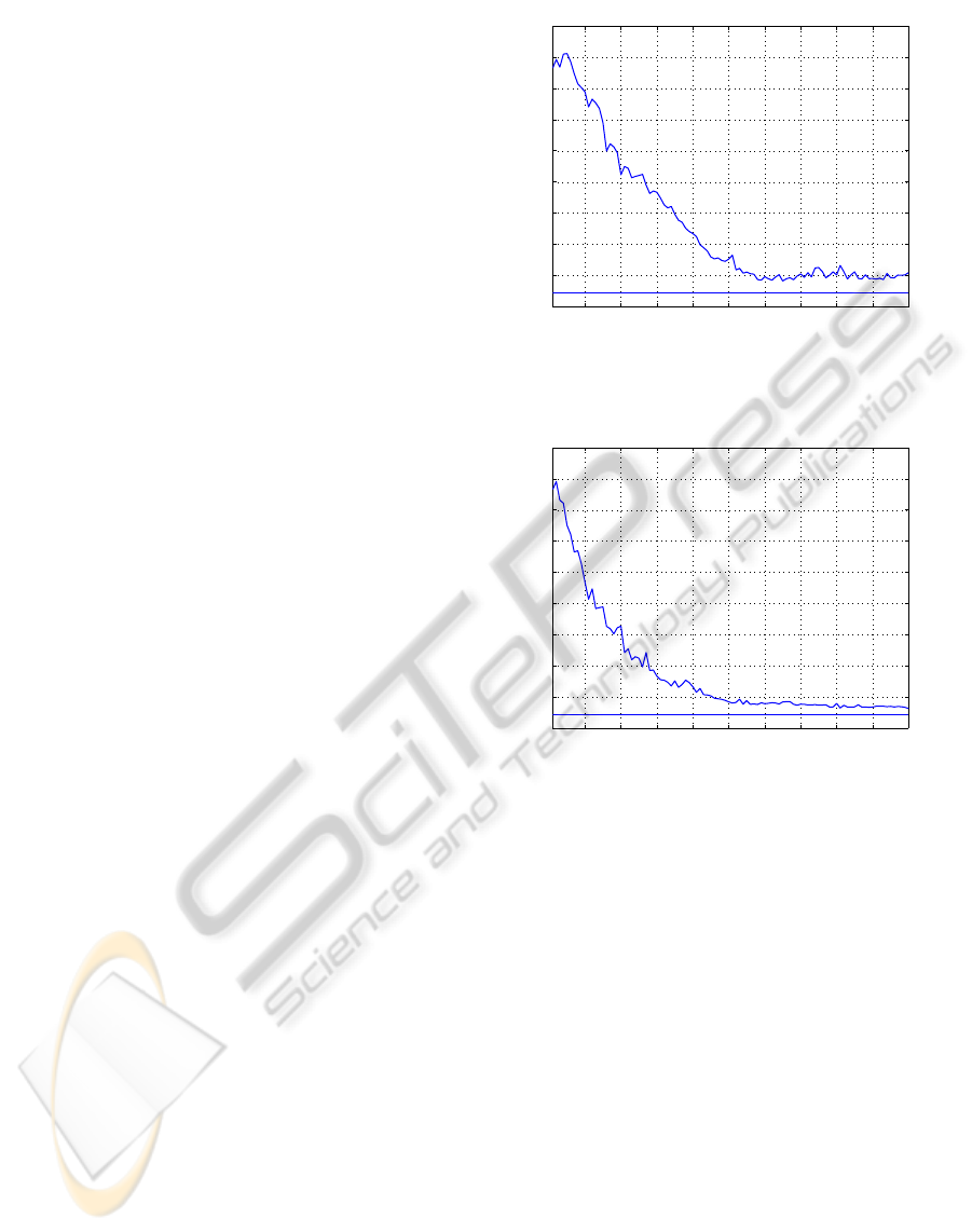
Figure 1 shows the performance of the learn-
ing system when using simply local updating. The
graphic corresponds to the average of 50 indepen-
dent experiments of 100 episodes each. The system
shows a stable performance after about 60 episodes,
and reaches a total accumulated cost of around 100.
The best performance obtained by exhaustive manual
tuning was near 44, and corresponds to the line at the
lower part of the figure. The best result obtained by a
single experiment test was 44.42. In average, the to-
tal number of Gaussians at the end of the experiments
was about 84.
In order to compare these results with those of
(Riedmiller, 2005b), we will take into account the
total number of times the system needs to be up-
dated with a sample to achieve the control. Riedmiller
reports that the swing-up and balance task required
100 iterations of the NFQ algorithm, each one re-
quiring 1000 epochs of batch learning with the Rprop
learning algorithm to train the neural net with an un-
specified number D of samples. This gives a total
of 100,000 × D sample updates. In our case, good
control is obtained after approximately 60 × 500 =
30,000 updates, which is significantly better.
These results were obtained with the simply lo-
10 20 30 40 50 60 70 80 90 100
0
100
200
300
400
500
600
700
800
900
episodes (x 500 iterations)
Accumulated cost
Figure 1: Average over 50 experiments of the accumulated
cost, on tests of 30 seconds, with simply local updating.
10 20 30 40 50 60 70 80 90 100
0
100
200
300
400
500
600
700
800
900
episodes (x 500 iterations)
Accumulated cost
Figure 2: Average over 50 experiments of the accumulated
cost, on tests of 30 seconds, with exponentially local updat-
ing.
cal updating of formula (13), which is sensible to the
effect of the biased sampling. Despite being good
results, we observe that the learning curve presents
some fluctuations that prevent the system to converge
to a value nearer to the theoretical optimum. Such
fluctuations are caused by transient learning phases
during which the system is not able to swing the pen-
dulum up, until a good policy is recovered again. This
is precisely the problem we anticipated: as far as the
system stabilizes near a good policy, it experiences
samples mostly near the optimal policy, so that the Q
estimation of less experienced actions degrades, and
eventually, suboptimal actions gain temporary control
until the system relearns their correct value. This is
the reason by which we introduced the exponent w
t,i
in the update formula (18) for exponentially local up-
dating. Its effectiveness is shown in Figure 2.
Results show that exponentially local updating
achieves convergence slightly faster and with a much
ICINCO 2010 - 7th International Conference on Informatics in Control, Automation and Robotics
166
0 0.5 1 1.5 2 2.5 3 3.5
−10
−8
−6
−4
−2
0
2
4
6
8
θ
θ
•
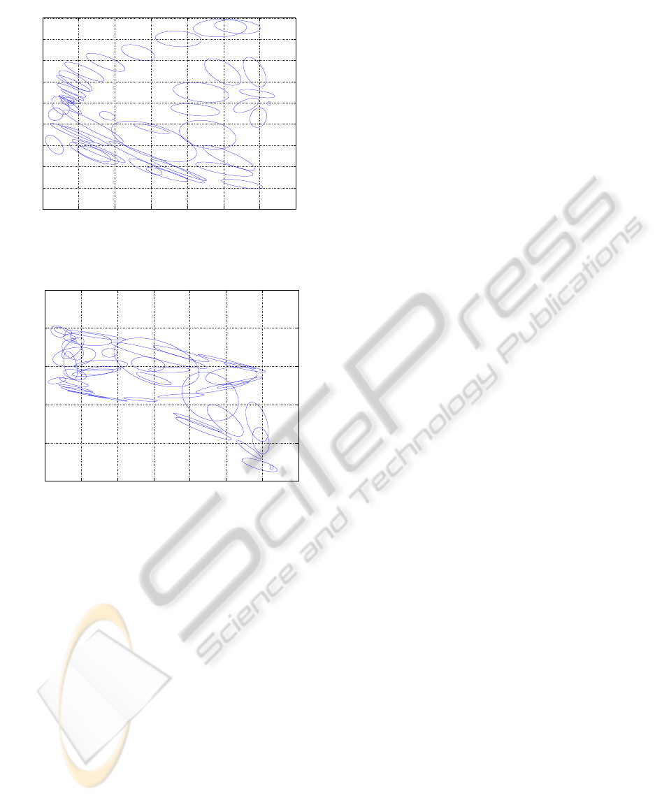
Figure 3: Distribution of Gaussians in a projection of the
joint space to the state space.
0 0.5 1 1.5 2 2.5 3 3.5
−20
−15
−10
−5
0
5
θ
q
Figure 4: Distribution of Gaussians in a projection of the
joint space to the (θ,q) space.
more stable behavior. In this case the average cost is
reduced to near 64, that is just 20 above the theoreti-
cal optimum, which compared with the 100− 44= 56
of the simply local updating corresponds to an im-
provement by a factor between 2 and 3. The number
of Gaussians used in this case is also lowered to less
than 60, in average. To check the effectiveness of ex-
ponentially local updating to prevent forgetting, we
observe that in the course of the 50 experiments, the
system failed to swing-up the pendulum after the 50th
episode only in a single occasion, compared with far
more that 30 with simply local updating.
Figures 3 and 4 show two projections of the Gaus-
sians of a typical GMM obtained for this problem af-
ter training. It can be seen that they are not equally
distributed along the whole configuration space, but
concentrate in the most common trajectories of the
system, what constitutes an efficient use of resources.
8 CONCLUSIONS
We proposed a new approach for Q-Learning in con-
tinuous state-action spaces, in which a Gaussian Mix-
ture Model that estimates the probability density in
the joint state-action-Qvalue space is used for func-
tion approximation. From this joint distribution we
can obtain, not just the expected value of Q for a given
state and action, but a full probability distribution that
is used to define a directed exploration-exploitation
strategy. As a further benefit, from the density estima-
tion in the joint space we can also obtain the sampling
density in the state-action space. This information is
used to remedy the problem of biased sampling inher-
ent to on-line Reinforcement Learning. For this, we
modified the incremental updating rule of an on-line
EM algorithm in order to avoid forgetting data of less
frequently sampled regions, even when exploration is
reiteratively done near the goal configurations.
Tests performed on a classical RL problem, the
swing-up and balance of an inverted pendulum, show
that our approach improves the results of previous
works when considering the number of sample up-
dates required to achieve the goal. The comparison
between our basic approach, using simply local up-
dating, and the proposed improvement using expo-
nentially local updating, shows that the approach is
effective in reducing the perturbing effect of biased
sampling.
Finally, we want to point out that the information
provided by the density estimation has not been fully
exploited yet. We expect to use the density informa-
tion in future works to better guide exploration during
learning.
ACKNOWLEDGEMENTS
This research was partially supported by Consolider
Ingenio 2010, project CSD2007-00018.
REFERENCES
Arandjelovic, O. and Cipolla, R. (2005). Incremental learn-
ing of temporally-coherent gaussian mixture models.
In Technical Papers - Society of Manufacturing Engi-
neers (SME).
Bellman, R. and Dreyfus, S. (1962). Applied Dynamic
Programming. Princeton University Press, Princeton,
New Jersey.
Bishop, C. M. (2006). Pattern Recognition and Ma-
chine Learning (Information Science and Statistics).
Springer-Verlag New York, Inc., Secaucus, NJ, USA.
REINFORCEMENT LEARNING FOR ROBOT CONTROL USING PROBABILITY DENSITY ESTIMATIONS
167

Dearden, R., Friedman, N., and Russell, S. (1998).
Bayesian q-learning. In In AAAI/IAAI, pages 761–768.
AAAI Press.
Dempster, A., Laird, N., Rubin, D., et al. (1977). Maxi-
mum likelihood from incomplete data via the EM al-
gorithm. Journal of the Royal Statistical Society. Se-
ries B (Methodological), 39(1):1–38.
Doya, K. (2000). Reinforcement learning in continuous
time and space. Neural Comput., 12(1):219–245.
Duda, R. O., Hart, P. E., and Stork, D. G. (2001). Pattern
classification. John Wiley and Sons, Inc, New-York,
USA.
Engel, Y., Mannor, S., and Meir, R. (2005). Reinforcement
learning with gaussian processes. In ICML ’05: Pro-
ceedings of the 22nd international conference on Ma-
chine learning, pages 201–208, New York, NY, USA.
ACM.
Ernst, D., Geurts, P., and Wehenkel, L. (2005). Tree-based
batch mode reinforcement learning. J. Mach. Learn.
Res., 6:503–556.
Figueiredo, M. (2000). On gaussian radial basis func-
tion approximations: Interpretation, extensions, and
learning strategies. Pattern Recognition, International
Conference on, 2:618–621.
Ghahramani, Z. and Jordan, M. (1994). Supervised learn-
ing from incomplete data via an em approach. In Pro-
ceeding of Advances in Neural Information Process-
ing Systems (NIPS’94), pages 120–127. San Mateo,
CA: Morgan Kaufmann.
Gordon, G. J. (1995). Stable function approximation in dy-
namic programming. In ICML, pages 261–268.
Neal, R. and Hinton, G. (1998). A view of the em algorithm
that justifies incremental, sparse, and other variants. In
Proceedings of the NATO Advanced Study Institute on
Learning in graphical models, pages 355–368, Nor-
well, MA, USA. Kluwer Academic Publishers.
Nowlan, S. J. (1991). Soft competitive adaptation: neural
network learning algorithms based on fitting statisti-
cal mixtures. PhD thesis, Pittsburgh, PA, USA.
Ormoneit, D. and Sen, S. (2002). Kernel-based reinforce-
ment learning. Machine Learning, 49(2-3):161–178.
Rasmussen, C. and Kuss, M. (2004). Gaussian processes in
reinforcement learning. Advances in Neural Informa-
tion Processing Systems, 16:751–759.
Riedmiller, M. (2005a). Neural fitted Q iteration-first ex-
periences with a data efficient neural reinforcement
learning method. Lecture notes in computer science,
3720:317–328.
Riedmiller, M. (2005b). Neural Reinforcement Learning to
Swing-up and Balance a Real Pole. In Proceedings of
the 2005 IEEE International Conference on Systems,
Man and Cybernetics, volume 4, pages 3191–3196.
Rottmann, A. and Burgard, W. (2009). Adaptive au-
tonomous control using online value iteration with
gaussian processes. In Proceedings of the 2009 IEEE
International Conference on Robotics and Automation
(ICRA’09), pages 2106–2111.
Sato, M.-A. and Ishii, S. (2000). On-line em algorithm for
the normalized gaussian network. Neural Comput.,
12(2):407–432.
Song, M. and Wang, H. (2005). Highly efficient incremental
estimation of gaussian mixture models for online data
stream clustering. In Proceedings of SPIE: Intelligent
Computing: Theory and Applications III, pages 174–
183, Orlando, FL, USA.
Sutton, R. and Barto, A. (1998). Reinforcement Learning:
An Introduction. MIT Press, Cambridge, MA.
Watkins, C. and Dayan, P. (1992). Q-learning. Machine
Learning, 8(3-4):279–292.
ICINCO 2010 - 7th International Conference on Informatics in Control, Automation and Robotics
168
