
A
PASSIVITY-BASED APPROACH TO DEPLOYMENT IN
MULTI-AGENT NETWORKS
Heath LeBlanc, Emeka Eyisi, Nicholas Kottenstette, Xenofon Koutsoukos and Janos Sztipanovits
Institute for Software Integrated Systems (ISIS), Vanderbilt University, 2015 Terrace Place, Nashville, TN 37203, U.S.A.
Keywords:
Passivity, Compositionality, Deployment, Overlay network, Input-output stability, Distributed protocol.
Abstract:
Surveillance and convoy tracking applications often require groups of networked agents for redundancy and
better coverage. An important goal upon deployment is to establish a formation around a target. Although there
exist distributed algorithms using only local communication that achieve this goal, they typically ignore desta-
bilizing effects resulting from implementation uncertainties, such as network delays and data loss. This paper
resolves these issues by introducing a discrete-time distributed design framework that uses a compositional,
passivity-based approach to ensure l
m
2
-stability regardless of overlay network topology, in the presence of net-
work delays and data loss. For the restricted case of a uniform node degree in the overlay network topology,
the paper shows that asymptotic formation establishment is achieved. Finally, simulations of velocity-limited
unmanned air vehicles (UAVs) are presented that demonstrate the robustness of the network architecture to
network delays and data loss.
1 INTRODUCTION
Modern surveillance and convoy tracking applica-
tions often require deploying groups of unmanned
aerial vehicles (UAVs). The benefit of using multi-
ple UAVs is redundancy, which reduces the likelihood
of missing interesting events on the ground, in the
presence of obstructions caused by nonuniform ter-
rain, vegetation, or man-made structures. Further, the
additional UAVs provide greater breadth of coverage.
A central task for such multi-agent systems is to es-
tablish a formation around an area of interest. For
example, an n-gon with a target as its center, at the
appropriate radius, may simultaneously provide sig-
nificant redundancy and breadth of coverage.
Performing coordinated tasks in multi-
agent systems using only local information has
been studied extensively over the past decade
(Olfati-Saber et al., 2007), (Ren et al., 2005),
(Olfati-Saber, 2006). Typically, in group coordi-
nation the desired formation emerges from the design
of the control law. In (Fax and Murray, 2004), the
so-called information filter is used for formation sta-
bility of LTI systems. For coordination of nonlinear
systems, contraction theory with wave variable com-
munication (Wang and Slotine, 2006), explicit design
of Lyapunov vector fields (Lawrence et al., 2008),
and passivity (Arcak, 2007), (Ihle et al., 2007),
(Bai et al., 2008), (Igarashi et al., 2008), have been
used successfully.
Much of the above work - especially the passivity-
based methods - has considered continuous-time
systems; however, for implementation discrete-
time design is needed. In addition, implementa-
tion uncertainties such as network delays and data
loss must be taken into consideration. This pa-
per focuses on decoupling the control design and
discrete-time implementation by using a passivity-
based framework inspired by work in telemanip-
ulation (Chopra et al., 2008), port-Hamiltonian sys-
tems (Stramigioli et al., 2005), and network control
(Kottenstette et al., 2009).
The unifying concept in the aforementioned work
is the scattering formalism, which has traditionally
been applied to power variables (effort and flow)
while closing the loop on velocity. In this work, the
scattering formalism is used abstractly (without the
physical interpretation) to close the loop on position.
The contributions of this paper are three-fold.
First, we introduce a compositional network control
system (NCS) design approach that guarantees pas-
sivity of the networked system. Secondly, we show
that the coupled multi-agent network is l
m
2
-stable for
any bidirectional overlay network with asymmetric
53
LeBlanc H., Eyisi E., Kottenstette N., Koutsoukos X. and Sztipanovits J. (2010).
A PASSIVITY-BASED APPROACH TO DEPLOYMENT IN MULTI-AGENT NETWORKS.
In Proceedings of the 7th International Conference on Informatics in Control, Automation and Robotics, pages 53-62
DOI: 10.5220/0002951500530062
Copyright
c
SciTePress

delays whenever the input-output mapping of each
agent is strictly-output passive. The stability re-
sult holds for packet-switched networks using easily
enforced constraints. Thirdly, for the single-input,
single-output (SISO) case, we perform steady-state
analysis and we show that the multi-agent network
can establish an n-gon upon deployment. Finally, we
provide simulations using Simulink/TrueTime to il-
lustrate the approach for controlling velocity-limited
quadrotor UAVs. Simulink is a graphical user envi-
ronment (GUI) used for the modeling, simulation, and
analysis of dynamical systems (MathWorks, 2008).
TrueTime extends Simulink with platform related
modeling concepts (i.e., networks, clocks, sched-
ulers) and supports simulation of networked and em-
bedded control systems with implementation effects
(Ohlin et al., 2007).
The rest of the paper is organized as follows: Sec-
tion 2 provides the formal problem statement and
other preliminaries. The distributed NCS design
framework is introduced in Section 3. The main the-
oretical results are detailed in Section 4. Section 5
presents simulations in Simulink/TrueTime illustrat-
ing our results. Finally, Section 6 provides concluding
remarks and future work.
2 PRELIMINARIES
Consider the problem of n agents establishing a for-
mation around a target in R
2
. Assume a global inertial
coordinate system and suppose the starting positions
of the agents are arbitrary. The goal is to establish
an n-gon, where the n agents tend to the coordinates
of the vertices asymptotically. Formally, we assign a
vertex ν
i
of the n-gon to agent i, with position x
i
(k),
i = 1,2,. .. ,n. Then we require
lim
k→∞
kx
i
(k) −ν
i
k
2
= 0. (1)
We consider a network of n interacting agents with
communication topology described by a connected
undirected graph, G = (V,E), where V = {1,2,...,n}
describes the agents and E ⊂V ×V models the bidi-
rectional communication. Additionally, each bidirec-
tional link may have asymmetric, time-varying de-
lays. The delays are denoted d
i j
(k) for link (i, j) ∈ E.
For the purpose of analysis, it is useful to intro-
duce the adjacency matrix, A = [a
i j
], associated with
graph G (Godsil and Royle, 2001). For an undirected
graph, the adjacency matrix is a symmetric matrix
(i.e., A = A
T
), and is mathematically defined by
a
i j
=
(
1 (i, j) ∈E;
0 (i, j) /∈ E.
(2)
Additionally, we define the set of neighbors, N
i
, of a
node i as those nodes which send messages to i, given
by N
i
= {j ∈V |a
ji
6= 0}. Finally, we denote the num-
ber of neighbors by |N
i
| = n
i
.
The agents communicate and process signals in
the extended
l
2
-space of functions that map
N
∪{
0
}
to R
m
, denoted l
m
2e
, which are mapped onto l
m
2
by the
truncation operator defined by
( f )
N
=
(
f (k) 0 ≤ k ≤ N −1;
0 otherwise.
(3)
Further, for all f , g ∈ l
m
2e
define
hf , gi
N
,
N−1
∑
k=0
f
T
(k)g(k). (4)
We use definitions for l
m
2
-stability and passiv-
ity for discrete-time systems, which are anal-
ogous to the continuous-time counterparts in
(van der Schaft, 1999):
Definition 1. Given a discrete-time system defined by
its input-output mapping, G : l
m
2e
→ l
m
2e
, the discrete-
time system is l
m
2
-stable if
u ∈ l
m
2
=⇒ G(u) ∈ l
m
2
. (5)
Definition 2. Let G: l
m
2e
→ l
m
2e
. Then, for all u ∈l
m
2e
:
1. G is passive if there exists some constant β ∈ R
(called the bias) such that
hG(u),ui
N
≥ −β, ∀N ∈ N; (6)
2. G is strictly output passive if there exists some
constants β ∈ R and ε > 0 such that
hG(u),ui
N
≥ εk(G(u))
N
k
2
2
−β, ∀N ∈ N. (7)
We assume a synchronous network, with period
T .
1
Further, each agent shares information only lo-
cally (no global shared resources). However, the de-
sired setpoints are calculated prior to deployment. Fi-
nally, the agents begin execution at time index k = 0.
3 NCS DESIGN
This section details the distributed network control
system (NCS) design. The objective is to provide
a passive-by-construction, discrete-time multi-agent
network. In general, the overlay network is bidi-
rectional with asymmetric delays. For simplicity,
consider the three node network shown in Figure 1.
1
We assume the agents use a clock synchronization
algorithm prior to deployment to ensure this assumption
holds.
ICINCO 2010 - 7th International Conference on Informatics in Control, Automation and Robotics
54
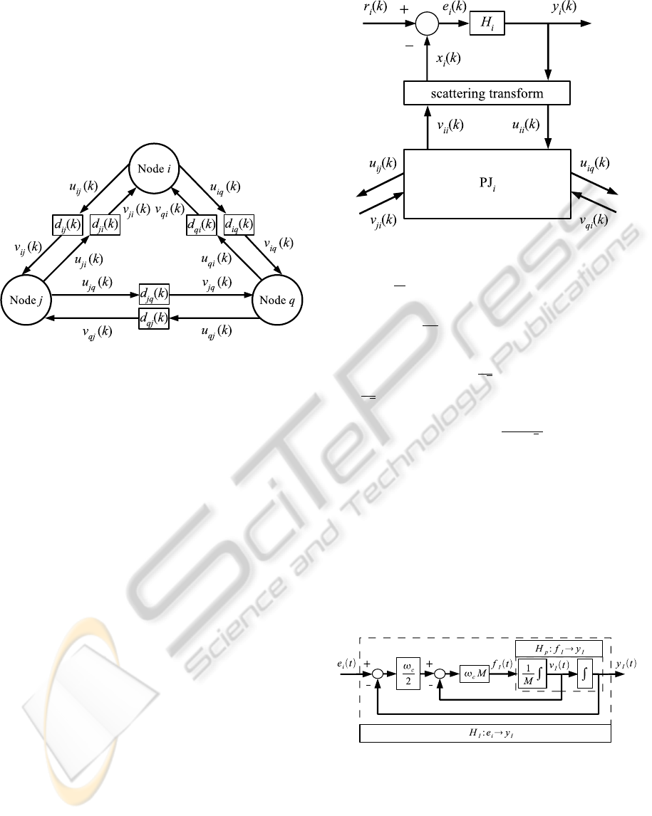
Each node represents a UAV, with each edge model-
ing the communication between UAVs. Realistically,
each link in the network is subject to delay imposed
by packet handling and transmission delays. This
is modeled by the time-varying delays (e.g., d
i j
(k)),
shown in Figure 1. The u and v variables in the fig-
ure are power wave variables, which are described in
Section 3.2.
Figure 1: A three node network with time-varying delays in
the communication links.
3.1 Agent Model
The agent model is shown in Figure 2. Each agent i
receives an input reference, r
i
, which influences the
output, y
i
, of the agent through the system mapping,
H
i
. H
i
describes a compensated plant, and is re-
quired to be strictly output passive. The variables x
i
and y
i
are transformed into the wave domain through
the scattering transformation. The node’s wave vari-
ables u
ii
and v
ii
are coupled to other nodes through
a power junction, PJ
i
, which allows two or more sys-
tems to be connected in a passivity-preserving manner
(Kottenstette et al., 2009). The scattering transforma-
tion and power junction are crucial to ensuring pas-
sivity of the networked system and will be described
in the next section.
For simplicity, we model the UAVs with a point
mass along two dimensions. We denote the point
mass system, H
p
: f
I
→ y
I
, in which f
I
∈ R
2
is the
inertial control force and y
I
∈ R
2
is the inertial posi-
tion as depicted in Figure 3. The equations of motion
are
˙y
I
(t) = v
I
(t)
M ˙v
I
(t) = f
I
(t).
Using the point mass model for each agent i, we
design an inertial position control system, which we
denote H
I
: e
i
→y
I
, shown in Figure 3. The inner loop
gain of the compensator is ω
c
M (ω
c
> 0) and the outer
Figure 2: Node architecture.
loop gain
ω
c
2
. The overall equation of motion
¨y
I
= −ω
c
˙y
I
−
ω
2
c
2
(y
I
−e
i
) = −2ζω
n
˙y
I
−ω
2
n
(y
I
−e
i
)
clearly indicates a stable second order system with
natural frequency ω
n
=
ω
c
√
2
and damping coefficient
ζ =
1
√
2
, where y
I
= e
i
at steady state. It can be shown
that the inertial position control system is inside the
sector [a,1], where a = −
1
2(1+
√
2)
(Zames, 1966),
(Kottenstette and Porter, 2009). Therefore, the sys-
tem H
I
: e
i
→ y
I
is not strictly output passive; how-
ever, by adding a high-pass filter in parallel, the sys-
tem may be rendered strictly output passive, as de-
picted in Figure 4 (with c = 2). Since e
i
= y
i
=
y
I
at steady state, the inertial position of the sys-
tem may be directly controlled. This model is dis-
cretized using a bilinear-like transform, called the
inner-product equivalent sample and hold (IPESH)
transform, which preserves the conic properties of the
system (Kottenstette et al., 2009).
Figure 3: Inertial position control system.
3.2 Network Model
In distributed control applications the information
transmitted across the network has inherent physical
meaning. It is well known that transforming these
physical variables into the wave domain can preserve
A PASSIVITY-BASED APPROACH TO DEPLOYMENT IN MULTI-AGENT NETWORKS
55

Figure 4: Strictly output passive inertial position control
system.
passivity and stability for a single bidirectional con-
nection (Chopra et al., 2008) and for star networks
(Kottenstette et al., 2009). In this paper, we extend
these approaches to distributed networks with arbi-
trary overlay topology. The network model is dis-
tributed in the sense that all nodes in the network com-
municate only locally.
We formally define the scattering transformation
as follows. For each i ∈V , the scattering transforma-
tion produces power waves u
ii
(k) and v
ii
(k) defined
by
u
ii
(k) =
1
√
2b
i
(b
i
y
i
(k) + x
i
(k)), (9a)
v
ii
(k) =
1
√
2b
i
(b
i
y
i
(k) −x
i
(k)). (9b)
This definition is similar to the one in
(Niemeyer and Slotine, 2004), with the force and
velocity variables replaced with x
i
and y
i
. In general,
we place no restriction on the physical meaning of x
i
and y
i
; however, for our UAV model, x
i
and y
i
denote
position. The scattering transformation is treated
as a mathematical definition, with the characteristic
impedance, b
i
, having appropriate units for physical
consistency.
Next, we define the power junction, which allows
two or more systems to be connected in the wave do-
main in a passivity-preserving manner.
Definition 3. Fix m, p ∈ N, p ≥ 2. Then, a power
junction is a function f : l
mp
2e
→ l
mp
2e
, which satisfies
for all ξ ∈ l
mp
2e
and all k ∈Z
+
the inequality
ξ
T
(k)ξ(k) ≥ f (ξ(k))
T
f (ξ(k)). (10)
The vector ξ(k) in the definition of the power junc-
tion is formed by concatenating the p inputs in l
m
2e
into
a single mp-dimensional column vector. For analyz-
ing our network model, it is useful to pair the p in-
puts to their corresponding outputs in the output col-
umn vector, f (ξ(k)), and partition the set of pairs into
two disjoint sets S
in
and S
out
. These sets denote the
net flow of power into and out of the power junction,
respectively. Formally, for i ∈ S
in
and o ∈ S
out
, let
u
i
,v
o
∈ l
m
2e
denote the inputs and v
i
,u
o
∈ l
m
2e
denote
the outputs of the power junction. Then (10) may be
rewritten as
∑
i∈S
in
u
T
i
(k)u
i
(k) −v
T
i
(k)v
i
(k) ≥
∑
o∈S
out
u
T
o
(k)u
o
(k) −v
T
o
(k)v
o
(k).
(11)
We implement each node’s power junction as a
linear set of equations. Specifically, we use the fol-
lowing equations. For each i ∈V, j ∈N
i
, and k ∈ Z
+
,
the outgoing waves are computed as
u
i j
(k) =
1
√
n
i
u
ii
(k), (12a)
v
ii
(k) =
1
√
n
i
∑
j∈N
i
v
ji
(k). (12b)
Although the functional form of the power junc-
tion is not constrained to be linear, these equations
simplify the steady state analysis and exhibit a local
averaging behavior in regular networks. This can be
seen as follows. Consider the wave variables that in-
fluence the power junction at a given node i, shown
in Figure 5, and suppose n
i
= n
j
≡ η, ∀i, j ∈V (i.e.,
a regular network). Then, for each j ∈ N
i
, v
ji
(k) =
u
ji
(k −d
ji
(k)). Thus, an expression for v
ii
(k) is given
by
v
ii
(k) =
1
√
η
∑
j∈N
i
v
ji
(k)
=
1
√
η
∑
j∈N
i
u
ji
(k −d
ji
(k))
=
1
√
η
∑
j∈N
i
1
√
η
u
j j
(k −d
ji
(k))
=
1
η
∑
j∈N
i
u
j j
(k −d
ji
(k)).
Therefore, in regular networks, the input wave vari-
able, v
ii
(k), is the average of its neighbors’ delayed
output wave variables, u
j j
(k −d
ji
(k)), j ∈ N
i
.
Due to the presence of delays and data loss
some (or all) of the v
ji
(k) may not be received at
time k, in which case v
ji
(k) , 0. Handling de-
layed and dropped packets as null packets satisfies
the synchronous assumption and preserves passivity
(Chopra et al., 2008). Before proceeding to describe
the constraints on delayed and lost data, we prove our
claim that the implementation given by (12) satisfies
the definition of a power junction.
Lemma 1. The implementation defined by (12) satis-
fies the power junction constraint.
Proof: From the remarks following the power
junction definition, it is sufficient to show that (12)
satisfy (11). Clearly, a sufficient condition for satis-
fying (11) is to enforce the following constraints for
ICINCO 2010 - 7th International Conference on Informatics in Control, Automation and Robotics
56
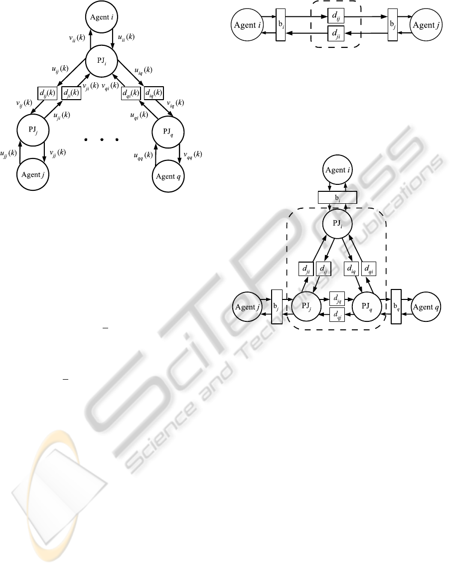
Figure 5: The neighbors of a node, showing the wave vari-
ables influencing the node through the power junction.
each component l = 1,2,...,m,
∑
j∈N
i
u
2
i j
l
(k) ≤u
2
ii
l
(k), (13a)
v
2
ii
l
(k) ≤
∑
j∈N
i
v
2
ji
l
(k), (13b)
where S
in
= {ii} and S
out
= {i j | j ∈N
i
}. To show that
(13a) is satisfied, we use (12a), which yields
∑
j∈N
i
u
2
i j
l
(k) =
∑
j∈N
i
1
n
i
u
2
ii
l
(k) = u
2
ii
l
(k).
For (13b) we combine (12b) with the Cauchy-
Schwartz inequality to get
v
2
ii
l
(k) =
1
n
i
(
∑
j∈N
i
v
ji
l
(k))
2
≤
∑
j∈N
i
v
2
ji
l
(k).
2
Finally, we constrain the network model by pre-
venting retransmission of data for each agent. Also,
as mentioned above, whenever receiver’s buffers are
empty, we process null packets. Based on these as-
sumptions, each channel (i, j) ∈ E satisfies the fol-
lowing inequality regardless of time-varying delays
and data loss (Chopra et al., 2008),
k(v
i j
)
N
k
2
2
≤ k(u
i j
)
N
k
2
2
, holds ∀N ∈N. (14)
This inequality states that each channel, viewed as the
input-output mapping shown in Figure 6, is passive.
4 ANALYSIS
4.1 Passivity of the Networked System
In this section we first prove that the network model
is passive and then show that the input-output map-
Figure 6: A point-to-point connection using the scattering
formalism to ensure passivity of the bidirectional connec-
tion subject to asymmetric time-varying delays, shown in-
side the dashed box.
ping describing the networked system is strictly out-
put passive. Figure 7 shows the passive network. The
following lemma proves that the portion inside the
dashed box of Figure 7 is passive.
Figure 7: A three node network illustrating the passive net-
work, shown inside the dashed box.
Lemma 2. Consider a network of n interacting dy-
namic systems constrained to the design framework
described in Section 3. Then, the global energy con-
straint
n
∑
i=1
{k(u
ii
)
N
k
2
2
−k(v
ii
)
N
k
2
2
} ≥ 0 (15)
is satisfied for all N ∈ N, regardless of time-varying
delays and data loss.
Proof: Sum the power constraints (11) of each
node i, with S
in
i
= {ii} and S
out
i
= {i j | j ∈ N
i
}, from
time k = 0 to k = N −1 and sum the resulting inequal-
ities over all nodes (rearranging the terms in the sums
appropriately). Then, invoke (14) to obtain
n
∑
i=1
{k(u
ii
)
N
k
2
2
−k(v
ii
)
N
k
2
2
}
≥
n
∑
i=1
∑
j∈N
i
a
i j
{k(u
i j
)
N
k
2
2
−k(v
i j
)
N
k
2
2
}
≥ 0.
2
A PASSIVITY-BASED APPROACH TO DEPLOYMENT IN MULTI-AGENT NETWORKS
57

The energy constraint of (15) also implies that
collectively, the mapping from the x
i
to the y
i
, i =
1,. .. ,n, is passive (see Figure 2). To show this, con-
sider the following power constraint, which may eas-
ily be derived from (9a) and (9b)
1
2
(u
T
ii
(k)u
ii
(k) −v
T
ii
(k)v
ii
(k)) = y
T
i
(k)x
i
(k). (16)
Substitute (16) into (15) to obtain
n
∑
i=1
hy
i
,x
i
i
N
≥ 0. (17)
Define x(k) and y(k) as the nm ×1 column vectors
formed by concatenating the x
i
(k) and y
i
(k), respec-
tively, of each node. Then, it follows that
hy,xi
N
≥ 0,
which satisfies the definition of passivity (6), with β =
0.
We conclude the section by proving that the entire
networked system (e.g., the three node system in Fig-
ure 7) is strictly output passive for arbitrary network
topologies.
Theorem 1. Consider a network of n interacting dy-
namic systems constrained to the design framework
described in Section 3. Define r(k) and y(k) as the
nm ×1 column vectors formed by concatenating the
r
i
(k) and y
i
(k), respectively, of each node. Finally,
define the input-output mapping H : l
nm
2e
→ l
nm
2e
such
that H(r(k)) = y(k). Then, H is strictly output pas-
sive.
Proof: Since each H
i
is strictly output passive,
there exists ε
i
> 0 and β
i
, for all i ∈V , such that
hy
i
,e
i
i
N
≥ ε
i
k(y
i
)
N
k
2
2
−β
i
. (18)
Making the substitution, x
i
(k) = r
i
(k)−e
i
(k) into (17)
and using the linearity of the inner-product, gives
n
∑
i=1
hy
i
,r
i
i
N
≥
n
∑
i=1
hy
i
,e
i
i
N
. (19)
Substituting (18) into (19) yields
n
∑
i=1
hy
i
,r
i
i
N
≥ ε
n
∑
i=1
k(y
i
)
N
k
2
2
−β, (20)
where ε = min
i
{ε
i
} and β =
∑
n
i=1
β
i
. Finally, we
rewrite (20) as
hy,ri
N
≥ εk(y)
N
k
2
2
−β. (21)
2
4.2 Stability
The previous result shows that the networked system
defined by the mapping H is strictly output passive. It
then follows that H is l
m
2
-stable.
Theorem 2. The mapping H(r(k)) = y(k) defined in
Theorem 1 is l
m
2
-stable.
Proof: We begin with the notion of finite l
m
2
-gain.
The map G has finite l
m
2
-gain if there exists finite con-
stants γ,β such that for all N ∈ N
k(G(u))
N
k
2
≤ γk(u)
N
k
2
+ β, ∀u ∈l
m
2e
. (22)
It is well known in continuous-time
(van der Schaft, 1999) and has been shown for
discrete-time (Kottenstette and Antsaklis, 2007) that
a sufficient condition for a system to have finite
l
m
2
-gain is for the system to be strictly output passive.
Therefore, by Theorem 1, H has finite l
m
2
-gain.
Now suppose u ∈ l
m
2
(i.e., kuk
2
< ∞). Then take
N →∞ in (22). This leads to
kG(u)k
2
≤ γkuk
2
+ β < ∞, ∀u ∈ l
m
2
.
Therefore, H(u) ∈l
m
2
. By Definition 1, H is l
m
2
-stable.
2
From the proof of Theorem 2, we see that any
system that is strictly output passive is necessarily
l
m
2
-stable. Therefore, each agent described by H
i
is
inherently stable. The benefit of the passivity-based
network framework is that it ensures that interactions
caused by the network do not destabilize the net-
worked multi-agent system. This result holds even in
the presence of time-varying delays and data loss (un-
der the assumptions outlined in Section 3.2) because
the passivity results hold. Moreover, the networked
multi-agent system will remain stable regardless of
network topology.
4.3 Steady-state Analysis
To analyze the behavior of the coupled multi-agent
system, we consider the system at steady-state. In
order to do this, we assume that each strictly output
system, H
i
, admits a steady-state solution whenever a
constant input is applied. With this assumption, there
exists a steady-state solution for the multi-agent sys-
tem (provided there is no data loss), since the rest of
the networked system is linear. For simplicity, we as-
sume the system is SISO. If the degrees of freedom of
the system are decoupled, this result may be applied
to MIMO systems.
Theorem 3. Consider a network of n interacting
SISO agents designed using the framework described
in Section 3 and ignore time delays and data loss. As-
sume the inputs, r
i
, reach steady-state and consider
ICINCO 2010 - 7th International Conference on Informatics in Control, Automation and Robotics
58

the outputs, y
i
, as k → ∞. If H
i
at each node i has
steady-state gain g
i
, then the steady-state output of
node i is given by
y
i
=
g
i
b
i
g
i
+1
"
r
i
+
√
2b
i
√
n
i
∑
j∈N
i
1
√
2b
j
n
j
[
b
j
g
j
−1
g
j
y
j
+ r
j
]
#
(23)
Proof: Since time delays and data loss are ig-
nored, we drop the time index. Using the relation
e
i
= r
i
−x
i
and replacing H
i
with g
i
, the input-output
relation y
i
= H
i
(e
i
) may be written as
y
i
= g
i
(r
i
−x
i
). (24)
Next, substituting (24) into (9b) and solving for x
i
yields
x
i
=
−
√
2b
i
b
i
g
i
+1
v
ii
+
b
i
g
i
b
i
g
i
+1
r
i
. (25)
Substituting (25) into (24) and reducing gives us
y
i
=
g
i
b
i
g
i
+1
r
i
+
√
2b
i
g
i
b
i
g
i
+1
v
ii
. (26)
Combining v
ji
= u
ji
with (12a) at node j (roles of j
and i are reversed), produces
v
ji
=
1
√
n
j
u
j j
.
Substituting this into (12b) for node i yields
v
ii
=
1
√
n
i
∑
j∈N
i
1
√
n
j
u
j j
. (27)
Now, solving (24) at node j for x
j
and substituting
into (9a) at node j produces
u
j j
=
1
√
2b
j
³
b
j
g
j
−1
g
j
y
j
+ r
j
´
(28)
Substitute (28) into (27) to get
v
ii
=
1
√
n
i
∑
j∈N
i
1
√
2b
j
n
j
³
b
j
g
j
−1
g
j
y
j
+ r
j
´
(29)
Finally, substitute (29) into (26) to obtain (23). 2
Theorem 3 provides a system of n equations de-
scribing the system asymptotically (as k → ∞). The
system of equations described by (23) are clearly cou-
pled and depend on the overlay network structure. For
the case of a regular topology, the following corol-
lary characterizes the system of equations and pro-
vides the means to precalculate the reference inputs
to asymptotically achieve a desired setpoint. For the
two-dimensional agent model described in Section
3.1 the two degrees of freedom are decoupled, so we
use this corollary to establish an n-gon around the tar-
get, as described in Section 2.
Corollary 1. Consider a network of n SISO agents
with a regular overlay network topology (i.e., n
i
=
n
j
≡ η ∀i, j ∈ V ). If all of the systems H
i
have iden-
tical steady-state gain g and each scattering trans-
formation has the same impedance b, the system of
steady-state equations may be written as
y =
g
bg+1
³
r +
1
η
A[
bg−1
g
y + r]
´
, (30)
where y and r are defined in Theorem 1 and A is
the adjacency matrix of the regular overlay network
topology. Assuming the inverse of (ηI + A) exists, we
may solve this equation for r to obtain
r =
1
g
(ηI + A)
−1
((bg + 1)ηI −(bg −1)A) y. (31)
5 SIMULATIONS
The experimental setup involves a network of eight
UAVs that communicate in a regular overlay network
topology, each with degree η = 4, and a synchronous
sampling period of T = 0.01 seconds. Each UAV
moves in the plane, influenced by its own input and
the wave variables received from its neighbors. We
model the UAVs as described in Section 3.1, so that
each has a steady state gain, g = 1, and characteris-
tic impedance, b = 1. The dynamics of the velocity
limited UAVs are implemented using Simulink mod-
els while TrueTime is used to simulate the network
dynamics and communication between neighboring
UAVs. The network protocol used is IEEE 802.11b,
with a speed of 11 Mbps.
5.1 Evaluation
We present five scenarios to demonstrate our design
framework.
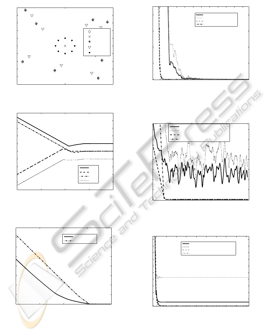
Experiment 1: Nominal Case. In this experiment,
delays and data loss are ignored. Figure 8a shows a
plot of the eight UAVs enclosing the target at the ori-
gin, within a radius of 100m. The data points show
the evolution of the UAVs from their initial positions
to their final positions. The UAVs cooperatively en-
close the target and each agent is 100m away from the
target, thus achieving the desired goal.
Figure 8b shows the x-positions of four agents
(UAVs 1, 3, 5, and 8) over a period of 200 seconds.
The desired x-positions for the four agents are 100m,
0m, 0m and -100m, respectively. These values corre-
spond to the desired configuration and are achieved in
about 160 seconds.
Figure 9 shows the average and maximum errors
of all the UAVs’ positions relative to the desired con-
figuration. From the figure, the average and maxi-
mum error reach the value of zero after 160 seconds
A PASSIVITY-BASED APPROACH TO DEPLOYMENT IN MULTI-AGENT NETWORKS
59
−500 0 500
−500
−400
−300
−200
−100
0
100
200
300
400
500
x−position(m)
y−position(m)
UAVs and Target Locations
y
I
at 0s
Target
y
I
at 1s
y
I
at 20s
y
I
at 200s
(a) UAVs and target positions.
0 50 100 150 200
−500
−400
−300
−200
−100
0
100
200
300
400
500
Time(S)
x−position(m)
Plot of UAVs’ x−positions
UAV1
UAV3
UAV5
UAV8
(b) Plot of UAVs’ x-position over time.
Figure 8: Network of UAVs (nominal case).
0 50 100 150 200
0
100
200
300
400
500
600
700
800
Time(s)
Error(m)
Average and Maximum Errors of UAV positions
Average Error
Maximum Error
Figure 9: Average and maximum errors of UAVs’ positions
(nominal case).
which corresponds to the time the UAVs achieve the
desired configuration.
Experiment 2: Nonuniform Constant Time De-
lays. This experiment demonstrates the robustness of
155 160 165 170 175 180 185 190 195 200 205
0
0.05
0.1
0.15
0.2
Time(s)
Error(m)
Average and Maximum Errors of UAV Positions
Average Error(Delay Case)
Maximum Error(Delay Case)
Average Error(Nominal Case)
Maximum Error(Nominal Case)
Figure 10: Average and maximum errors of UAVs’ po-
sitions (nonuniform constant delay in all communication
channels).
150 160 170 180 190 200
0
1
2
3
4
5
6
7
Time(s)
Error(m)
Average and Maximum Errors of UAV positions
Average Error(Packet Loss Case)
Maximum Error(Packet Loss Case)
Average Error(Nominal Case)
Maximum Error(Nominal Case)
Figure 11: Average and maximum errors of UAVs’ posi-
tions (ten percent probability of packet loss).
155 160 165 170 175 180 185 190 195 200
0
0.02
0.04
0.06
0.08
0.1
0.12
0.14
0.16
0.18
0.2
Time(s)
Error(s)
Average and Maximum Errors of UAV Positions
Average Error(Time−Varying Delay Case)
Maximum Error(Time−Varying Delay Case)
Average Error(Nominal Case)
Maximum Error(Nominal Case)
Figure 12: Average and maximum errors of UAVs’ posi-
tions (time-varying delay case).
the distributed network of UAVs to nonuniform con-
stant delays. We introduce nonuniform time delays,
between 1 to 10 seconds, in all the communication
channels of the network. Figure 10 shows the average
ICINCO 2010 - 7th International Conference on Informatics in Control, Automation and Robotics
60
130 140 150 160 170 180 190 200 210 220 230
0
5
10
15
20
25
30
35
Time(s)
Error(m)
Average and Maximum Errors of UAV Positions
Average Error( Combined Network Effects)
Maximum Error( Combined Network Effects)
Average Error(Nominal Case)
Maximum Error(Nominal Case)
Figure 13: Average and maximum errors of UAVs’ posi-
tions (time-varying delay and packet loss case).
−110−100−90 −80 −70 −60 −50 −40 −30 −20 −10 0 10 20 30 40 50 60 70 80 90 100 110
−110
−100
−90
−80
−70
−60
−50
−40
−30
−20
−10
0
10
20
30
40
50
60
70
80
90
100
110
x−position(m)
y−position(m)
UAVs and Target Locations
Figure 14: UAVs and target positions (time-varying delay
and packet loss case).
and maximum errors, comparing the nominal case to
the case with nonuniform constant delays. From the
figure, the average and maximum errors for the delay
case reach the value of zero after 200 seconds, taking
about 40 seconds more time than in the nominal case
to reach the desired configuration. The presence of
time delays in the network does not prevent the agents
from reaching the desired configuration; however, the
time delays increase the time it takes to reach the de-
sired configuration.
Experiment 3: Data Dropouts. This experiment
demonstrates the effect of packet loss on the behav-
ior of the UAVs. A probabilistic model is used to im-
plement the loss of packets in the channels. For our
studies, we simulate the case of a ten percent prob-
ability of packet loss. Figure 11 shows the average
and maximum errors, comparing the nominal case to
the case of ten percent probability of packet loss. The
plot shows that even with ten percent packet loss, the
UAVs still manage to come very close to the desired
configuration, demonstrating the resilience of the net-
work. Due to the packet loss, the UAVs will never
reach a steady state; however, the UAVs’ positions
end up within a maximum error of 6 meters and an
average error of 4 meters of the desired configuration.
Experiment 4: Time-varying Delays. This experi-
ment demonstrates the effect of time-varying delays
on the behavior of the UAVs. To simulate the case
of time-varying delays, we incorporate a disturbance
node in the network. The sampling period of the dis-
turbance node is set to a value of 0.05 seconds, and
the disturbance node floods the network with distur-
bance packets based on a Bernoulli process with pa-
rameter d. The disturbance node samples a uniformly
distributed random variable X[k] ∈ [0,1] every 0.05
seconds. If X[k] > d, a disturbance packet is forced on
the network. Figure 12 shows the average and maxi-
mum errors, comparing the nominal case to the time-
varying delay case, with d = 0.5. The plot shows that
in the presence of time-varying delays, the UAVs re-
main stable and settle within a maximum error of 0.09
meters and an average error of 0.02 meters from the
desired configuration.
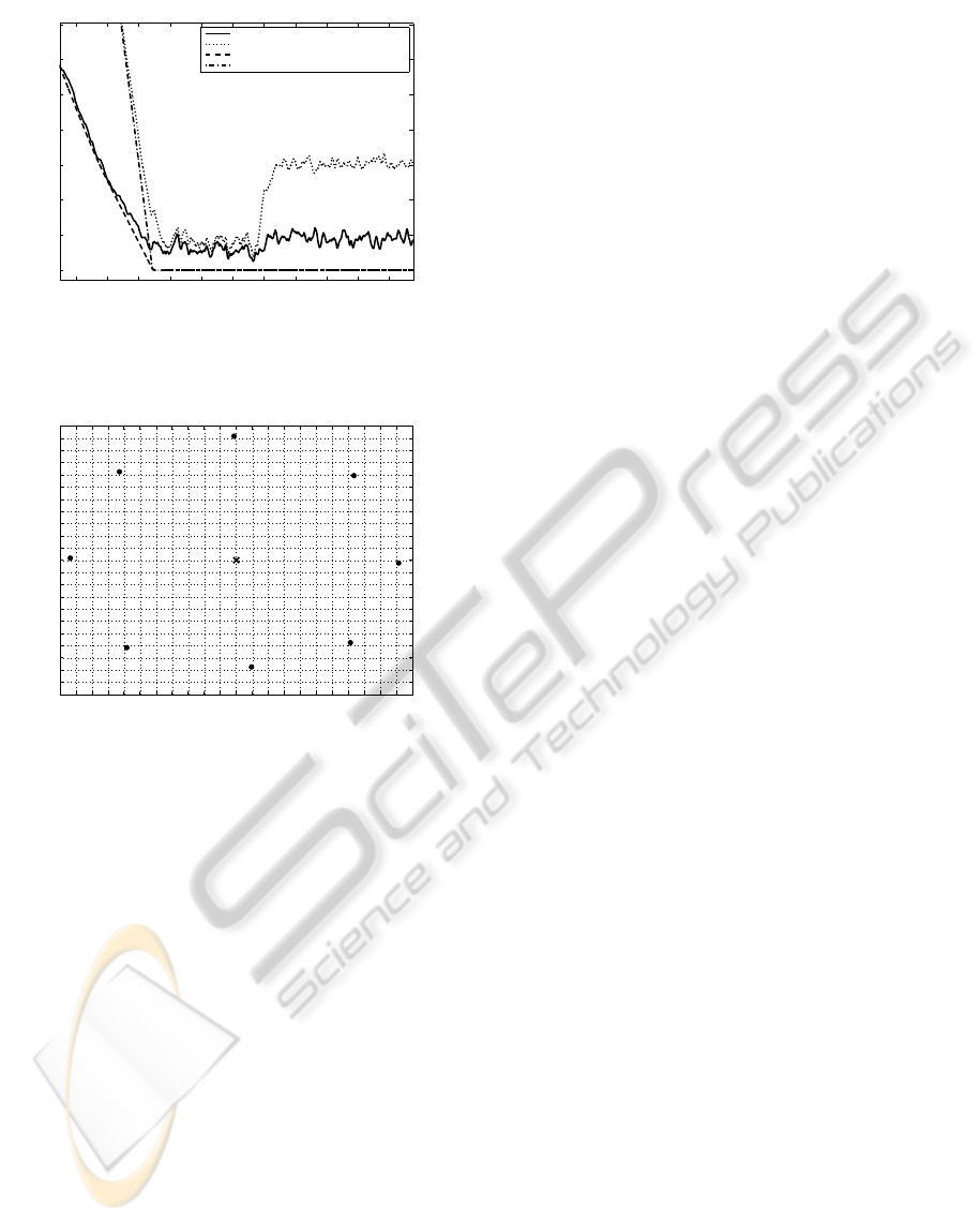
Experiment 5: Combined Network effects. The
experiment demonstrates the combined effects of ten
percent packet loss and time-varying delays on the be-
havior of the UAVs. This experiment studies the com-
bined network effects of time-varying delays and data
loss in order to simulate the real world dynamics of
the network. Again, the time-varying delays are intro-
duced through the disturbance node with d = 0.5. Fig-
ure 13 shows the average and maximum errors, com-
paring the nominal case to the case with the combined
network effects. The figure shows that the average
and maximum errors increase slightly after appearing
to settle near 5 meters. This occurs because one of the
UAVs actually moves interior to the circle around the
target, shown in Figure 14. The UAV directly below
the target is approximately 15 meters away from its
desired location, and causes the maximum error seen
in Figure 13.
6 CONCLUSIONS
Discrete-time implementation of networked multi-
agent systems introduces significant challenges
caused by effects such as network delays and data
loss. This paper proposes a passive-by-construction
distributed network control design framework that en-
sures l
m
2
-stability in the presence of these network ef-
fects. Using steady-state analysis, we show how to
control the agents in the multi-agent network in order
to establish an n-gon upon deployment. Simulations
supporting the theoretical results are presented on the
A PASSIVITY-BASED APPROACH TO DEPLOYMENT IN MULTI-AGENT NETWORKS
61

Simulink/TrueTime platform. In future work, we plan
to extend the design framework to achieve other group
oriented tasks such as output synchronization, forma-
tion control, and rendezvous. We will also extend the
work to formations in R
3
.
ACKNOWLEDGEMENTS
This work is supported in part by the National Sci-
ence Foundation (NSF CCF-0820088), the U.S. Army
Research Office (ARO W911NF-10-1-0005), the
U.S. Air Force Office of Scientific Research (MURI
FA9550-06-0312), the U.S Army Research Labo-
ratory (ARL W911NF-087-2-0004), and Lockheed-
Martin. The views and conclusions contained herein
are those of the authors and should not be interpreted
as necessarily representing the official policies or en-
dorsements, either expressed or implied, of the U.S.
Government.
REFERENCES
Arcak, M. (2007). Passivity as a design tool for group co-
ordination. IEEE Transactions on Automatic Control,
52(8):1380–1390.
Bai, H., Arcak, M., and Wen, J. T. (2008). Rigid body atti-
tude coordination without inertial frame information.
Automatica, 44(12):3170 – 3175.
Chopra, N., Berestesky, P., and Spong, M. (2008). Bilat-
eral teleoperation over unreliable communication net-
works. IEEE Transactions on Control Systems Tech-
nology, 16(2):304–313.
Fax, J. A. and Murray, R. M. (2004). Information flow
and cooperative control of vehicle formations. IEEE
Transactions on Automatic Control, 49(9):1465 –
1476.
Godsil, C. and Royle, G. (2001). Algebraic Graph Theory.
Springer-Verlag New York, Inc.
Igarashi, Y., Hatanaka, T., Fujita, M., and Spong, M. (2008).
Passivity-based output synchronization in se(3). In
American Control Conference, pages 723–728.
Ihle, I.-A. F., Arcak, M., and Fossen, T. I. (2007). Passivity-
based designs for synchronized path-following. Auto-
matica, 43(9):1508 – 1518.
Kottenstette, N. and Antsaklis, P. (2007). Stable digital con-
trol networks for continuous passive plants subject to
delays and data dropouts. 46th IEEE Conference on
Decision and Control, pages 4433–4440.
Kottenstette, N., Hall, J., Koutsoukos, X., Antsaklis, P.,
and Sztipanovits, J. (2009). Digital control of mul-
tiple discrete passive plants over networks. Inter-
national Journal of Systems, Control and Communi-
cations (IJSCC): Special Issue on Progress in Net-
worked Control Systems. To Appear.
Kottenstette, N. and Porter, J. (2009). Digital Passive Atti-
tude and Altitude Control Schemes for Quadrotor Air-
craft. 7th International Conference on Control and
Automation.
Lawrence, D. A., Frew, E. W., and Pisano, W. J. (2008).
Lyapunov vector fields for autonomous uav flight con-
trol. AIAA Journal of Guidance, Control, and Dynam-
ics, 31(5):1220–1229.
MathWorks, I. T. (2008). Simulink. Dynamic System Simu-
lation for MATLAB, Version 7.1.
Niemeyer, G. and Slotine, J.-J. E. (2004). Telemanipulation
with time delays. International Journal of Robotics
Research, 23(9):873 – 890.
Ohlin, M., Henriksson, D., and Cervin, A. (2007).
TrueTime 1.5 Reference Manual. Dept. of
Automatic Control, Lund University, Sweden.
http://www.control.lth.se/truetime/.
Olfati-Saber, R. (2006). Flocking for multi-agent dynamic
systems: algorithms and theory. IEEE Transactions
on Automatic Control, 51(3):401–420.
Olfati-Saber, R., Fax, J. A., and Murray, R. M. (2007). Con-
sensus and cooperation in networked multi-agent sys-
tems. Proceedings of the IEEE, 95(1):215–233.
Ren, W., Beard, R., and Atkins, E. (2005). A survey of con-
sensus problems in multi-agent coordination. In Pro-
ceedings of the American Control Conference, pages
1859–1864 vol. 3.
Stramigioli, S., Secchi, C., van der Schaft, A. J., and Fan-
tuzzi, C. (2005). Sampled data systems passivity and
discrete port-hamiltonian systems. IEEE Transactions
on Robotics, 21(4):574 – 587.
van der Schaft, A. (1999). L2-Gain and Passivity in Nonlin-
ear Control. Springer-Verlag New York, Inc., Secau-
cus, NJ, USA.
Wang, W. and Slotine, J.-J. (2006). Contraction analysis of
time-delayed communications and group cooperation.
IEEE Transactions on Automatic Control, 51(4):712–
717.
Zames, G. (1966). On the input-output stability of time-
varying nonlinear feedback systems part one: Con-
ditions derived using concepts of loop gain, conicity,
and positivity. IEEE Transactions on Automatic Con-
trol, 11(2):228–238.
ICINCO 2010 - 7th International Conference on Informatics in Control, Automation and Robotics
62
