
ESTIMATION AND COMPENSATION OF DEAD-ZONE INHERENT
TO THE ACTUATORS OF INDUSTRIAL PROCESSES
Auciomar C. T. de Cequeira, Marcelo R. B. G. Vale, Daniel G. V. da Fonseca
Laboratory of Automation in Petroleum, Federal University of Rio Grande do Norte, Campus Universitário, Natal, Brazil
Fábio M. U. de Araújo, André L. Maitelli
Department of Computing and Automation, Federal University of Rio Grande do Norte, Natal, Brazil
Keywords:
Parameters estimation, Nonlinearity, Inverse compensation, Dead-zone, Hammerstein model.
Abstract:
The oscillations present in control loops can cause damages in industry. Canceling, or even preventing such
oscillations, would save up to large amount of dollars. Studies have identified that one of the causes of these
oscillations are the nonlinearities present on industrial processes actuators. This paper has the objective to
develop a methodology for removal of the harmful effects of nonlinearities. Will be proposed a parameters
estimation method to the Hammerstein model, whose nonlinearity is represented by dead-zone. The estimated
parameters will be used to construct the inverse model of compensation. A simulated level system was used
as test platform. The valve that controls inflow has a dead-zone. Results analysis shows an improvement on
system response.
1 INTRODUCTION
Inside industrial process there are hundreds of control
loops, which are mainly composed by sensors, actua-
tors, Programmable Logic Control (PLC) and Super-
visory Control and Data Acquisition (SCADA). The
control efficiency is, therefore, important to ensure
a high quality product and low cost production. So,
finding and solving control loop problems of a pro-
cess implies in reject reduction, better product ho-
mogeneity, lower production costs and higher rates
of production. Even an 1% energy or control effi-
ciency improvement means a huge economy in indus-
trial process, of millions of dollars (Desborough and
Miller, 2002).
Several studies related to control loop perfor-
mance indicate that the majority present deficient be-
havior, showing oscillations at process output. One of
those researches (Desborough and Miller, 2002) eval-
uated 26 thousand control loops and classified them
this way:
• 16% as excellent;
• 16% as acceptable;
• 22% as fair;
• 10% as poor;
• 36% as open loop.
Among the causes for this deficient performance
are included bad tune of controllers, wrong process
project, the incoming oscillatory perturbations and
the nonlinearities of the actuators. And those non-
linearities cause dead-band in actuators as well.
An audit made by a big producer of valves has
shown that 30% of the products presented about 4%
or more of dead-band and approximately 65% of the
valves had a dead-band higher than 2% (FISCHER,
2005). As most of the actions of regulatory control
consist of small variations in the order of 1% or less,
the control loops would not act effectively in the pro-
cess for responding to these small variations. For a
good performance, it is recommended that the con-
trol valve dead-band is about 1% or less (Campos and
Teixeira, 2007).
A point to mention is that 20 to 30% of the oscil-
lations in control loops are caused by nonlinearities
of the valves (Ulaganathan and Rengaswamy, 2008),
among which we can point out the static friction, hys-
teresis, backlash and dead-zone as the best known.
The compensation of the effects of such nonlineari-
ties would help in solving the problem of poor perfor-
62
C. T. de Cequeira A., R. B. G. Vale M., G. V. da Fonseca D., M. U. de Araújo F. and L. Maitelli A. (2010).
ESTIMATION AND COMPENSATION OF DEAD-ZONE INHERENT TO THE ACTUATORS OF INDUSTRIAL PROCESSES.
In Proceedings of the 7th International Conference on Informatics in Control, Automation and Robotics, pages 62-70
DOI: 10.5220/0002953000620070
Copyright
c
SciTePress

mance of about a quarter of the controllers present in
the industry.
The aim of this study is therefore to minimize or
cancel the oscillations observed in the outputs of in-
dustrial processes, which are caused by dead-zone in-
herent to the actuators of control loops.
The industrial processes were represented by the
Hammerstein model. Inverse models of nonlinearity
will be built based on dead-zone parameter estima-
tion. The intention is to make these inverse models
capable to compensate the nonlinearity, reducing the
oscillations and its harmful effects. It will be pro-
posed a method of parameter estimation for a Ham-
merstein model that contains as the non-linear part a
dead-zone.
2 MATHEMATIC MODELS
This section describes the mathematic models utilized
in dead-zone estimation and compensation methodol-
ogy. This methodology uses the Hammerstein model
to represent the industrial processes containing dead-
zone. Thereby, the linear part of Hammerstein model
is represented by Output Error model and the non-
linear part is represented by dead-zone. Besides the
Hammerstein model, this section also describes the
inverse model for dead-zone compensation. This one
will reduce prejudicial effects of nonlinearity.
It should be clear that the mathematic models de-
scribed in this section are simplified descriptions of
real physical phenomena.
2.1 Hammerstein Model
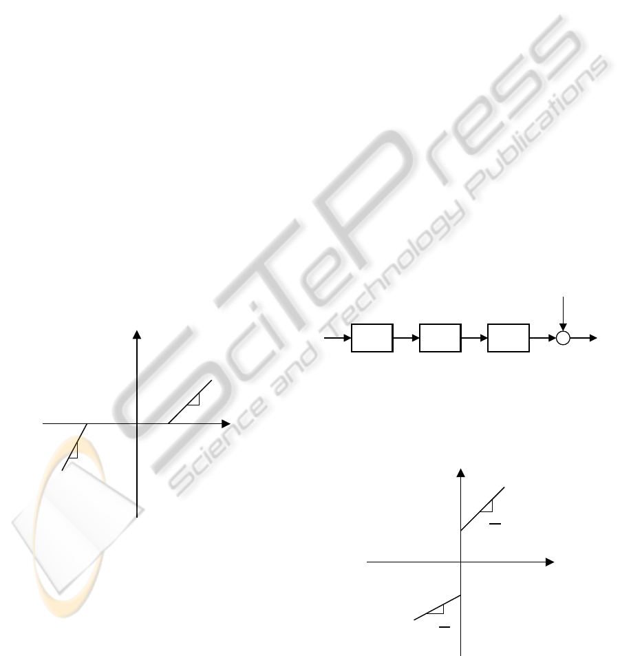
The nonlinear Hammerstein model is composed by
a static nonlinearity preceding a linear dynamic
(Aguirre, 2007). This model is called block-oriented
or block-structured model (Chen, 1995). Thus, both
the non-linearity and the dynamics are represented by
blocks, as shown in Figure 1. Here, the NL block
represents the static nonlinearity function and the L
block represents the linear dynamic of modeled pro-
cess. The signs u(k), y(k) and e(k) are the nonlin-
earity input, the output and the noise of the system,
respectively. The signal x(k) is called internal vari-
able of the Hammerstein model (nonlinearity output
and linear dynamic input), and, in general, it cannot
be measured, making it difficult to estimate the pa-
rameters in the same models.
Although very simple, this structure may repre-
sent several actual physical processes, such as indus-
trial processes with variable gain and control systems
NL L
u(k) x(k) y(k)
e(k)
+
+
Figure 1: Hammerstein model.
with linear processes and nonlinear actuators (the lat-
ter falls within the subject matter in this work). There-
fore Hammerstein models are popular in control engi-
neering.
2.2 Output Error Model
There are some mathematical representations that are
especially suitable for system identification, using
classic algorithms to the estimation of its parameters.
Along with the ARX and ARMAX models, the Out-
put Error model is one of the most used structures. In
this study, this model represents the linear dynamic of
the Hammerstein system (block L of Figure 1) and it
is represented in Figure 2. In the same model, it is as-
sumed that the noise disturbs the output in an additive
manner, as equations below.
y(k) = q
−d
B(q)
A(q)
x(k) + e(k) (1)
A(q)y(k) = q
−d
B(q)x(k) + A(q)e(k) (2)
A(q) and B(q) are polynomials of order n
a
and n
b
,
respectively, and are defined below. d represents the
pure delay system and q
−1
is the shift operator, so
x(k)q
−d
= x(k − d).
A(q) = 1+ a
1
q
−1
+ ... + a
n
q
−n
a
B(q) = b
0
+ b
1
q
−1
+ ... + b
m
q
−n
b
x(k)
B(q)
A(q)
y(k)
e(k)
+
+
Figure 2: Output Error model.
The Output Error model is much more realistic
than the ARX and ARMAX because the modeling of
noise does not include the dynamics of the process
1/A(q) (Nelles, 2000). So, the parameter estimation
task becomes more difficult. As shown in Equation
(2), the noise is not white but colored due to the pres-
ence of the polynomial A(q). For this reason, the least
squares method cannot be used. A non-polarized al-
gorithm should be used so that the estimation is not
biased.
ESTIMATION AND COMPENSATION OF DEAD-ZONE INHERENT TO THE ACTUATORS OF INDUSTRIAL
PROCESSES
63
The Equation (2) can be rewritten in the form of
summations, already introducing the delay in the in-
put signal.
y(k) =
n
b
∑
i=0
b
i
x(k− d − i) −
n
a
∑
j=1
a
j
y(k− j)
+
n
a
∑
j=1
a
j
e(k− j) + e(k)
(3)
The signals y(k), x(k) and e(k) are the same as
the Hammerstein model (Figure 1), and have been de-
fined previously.
2.3 Dead-zone
The dead-zone is a static nonlinearity with no mem-
ory that describes the insensitivity of components for
small signals. It can be seen as a static relationship be-
tween input and output signals, in which, for a range
of input values, there is no answer. Once the output
appears, the relationship between input and output is
linear.
Figure 3 shows a graphical representation of the
dead-zone, where u(k) is the input and x(k) is the out-
put. The limits b
r
and b
l
represent the range where
the output signal remains unchanged, and m
r
and m
l
indicate the slope of the lines. By definition b
r
> 0,
b
l
< 0, m
r
> 0 and m
l
> 0, and in general, neither the
limits nor the slopes are equal.
u(k)
x(k)
m
r
b
r
b
l
m
l
Figure 3: Dead-zone graphic.
Analytically, the dead-zone can be written as fol-
lows:
x(k) =
m
r
[u(k) − b
r
], if u(k) ≥ b
r
0, if b
l
< u(k) < b
r
m
l
[u(k) − b
l
], if u(k) ≤ b
l
(4)
One way to write the behavior of the dead-zone so
that it is linear in the parameters is:
x(k) = X
r
(k)m
r
[u(k) − b
r
] + X
l
(k)m
l
[u(k) − b
l
] (5)
where X
r
(k) and X
l
(k) are auxiliary functions that
take the value 0 (zero) or 1 (one) according to the fol-
lowing conditions:
X
r
(k) =
1, if u(k) ≥ b
r
0, otherwise
(6)
X
l
(k) =
1, if u(k) ≤ b
l
0, otherwise
(7)
2.4 Inverse Model for Dead-zone
Compensation
It is known that the nonlinearities are among the key
factors that limit the static and dynamic performance
of control systems, preventing high precisions when
using linear controllers. In order to cancel the harmful
effects generated by the dead-zone, it is proposed to
implement its inverse model.
The Figure 4 shows the structure used in this
work for the cancellation of this nonlinearity. The
inverse nonlinearity (INL block) was allocated be-
fore the nonlinearity (NL block) to cancel out its ef-
fects. When implemented with the real parameters,
such compensation cancels completely the effects of
dead-zone. Therefore, if the dead-zone is fully com-
pensated, the input signal u
c
(k) must be equal to the
signal x(k).
INL NL L
u(k) x(k)u
c
(k) y(k)
e(k)
+
+
Figure 4: Block diagram of nonlinearity compensation.
The graphical relationship between the input sig-
nal u
c
(k) and output signal u(k) is shown in Figure
5.
u
c
(k)
u(k)
1
m
r
1
m
l
b
r
b
l
Figure 5: Graphic of dead-zone inverse compensation.
ICINCO 2010 - 7th International Conference on Informatics in Control, Automation and Robotics
64

The dead-zone inverse model is represented by
Equation 8. The parameters b
r
, b
l
, m
r
and m
l
are the
same used in modeling of dead-zone.
u(k) =
1
m
r
[u
c
(k) + m
r
b
r
], if u
c
(k) > 0
0, if u
c
(k) = 0
1
m
l
[u
c
(k) + m
l
b
l
], if u
c
(k) < 0
(8)
For a linear parameterization of inverse compen-
sation, we have:
u(k) = χ
r
(k)
1
m
r
[u
c
(k) + m
r
b
r
]
+χ
l
(k)
1
m
l
[u
c
(k) + m
l
b
l
]
(9)
where χ
r
(k) and χ
l
(k) are auxiliary functions defined
as:
χ
r
(k) =
1, if u
c
(k) > 0
0, otherwise
(10)
χ
l
(k) =
1, if u
c
(k) < 0
0, otherwise
(11)
The inverse model equation is similar to the dead-
zone model. The variables m
r
, m
l
, b
r
and b
l
have the
same meaning of Equation (5). The difference lies in
the definition of auxiliary functions χ
r
(k) and χ
l
(k).
To check the accuracy of the inverse model, in
other words, to conclude that x(k) = u
c
(k), three sit-
uations will be analyzed: u
c
(k) > 0, u
c
(k) < 0 and
u
c
(k) = 0. For this proof, the function of the inverse
of the dead-zone will be called ZI(·).
Lemma 1. (Dead-zone Inverse) when implemented
with real parameters m
r
, m
l
, b
l
and b
r
, the dead-zone
inverse (8) cancels the effect of dead-zone (4), that is
u(k) = ZI(u
c
(k)) ⇒ x(k) = u
c
(k),∀k ≥ 0.
Proof. Suppose u
c
(k) > 0. For u
c
(k) > 0, the auxil-
iary function χ
r
(k) (10) will be equal to 1 and χ
l
(k)
(11) will take value 0. Therefore, u(k) (9) will be:
u(k) =
1
m
r
[u
c
(k) + m
r
b
r
] =
u
c
(k)
m
r
+ b
r
(12)
As it was admitted that u
c
(k) > 0, and by definition
m
r
> 0, the portion
u
c
(k)
m
r
is also positive. So, u(k) >
b
r
. The auxiliary function X
r
(k) (6) will take value
1, while X
l
(k) (7) will be 0. Substituting (12) in (5)
with the appropriate values of the auxiliary functions
we have:
x(k) = m
r
u
c
(k)
m
r
+ b
r
− b
r
(13)
Making the simplifications, we conclude that x(k) =
u
c
(k).
Suppose that u
c
(k) < 0. For u
c
(k) < 0, the auxil-
iary function χ
r
(k) (10) will be equal to 0 and χ
l
(k)
(11) will take value 1. As a result, u(k) (9) will be:
u(k) =
u
c
(k) + m
l
b
l
m
l
=
u
c
(k)
m
l
+ b
l
(14)
As it was admitted that u
c
(k) < 0, and by defini-
tion m
l
> 0, the portion
u
c
(k)
m
r
will be negative. So,
u(k) < b
l
. The auxiliary function X
r
(k) (6) will take
value 0 while X
l
(k) (7) will be equal to 1. Substituting
(14) in (5) with the appropriate values of the auxiliary
functions we have:
x(k) = m
l
u
c
(k)
m
l
+ b
l
− b
l
(15)
Making the simplifications, we conclude that x(k) =
u
c
(k).
Suppose that u
c
(k) = 0. For u
c
(k) = 0, the auxil-
iary functions χ
r
(k) (10) and χ
l
(k) (11) are equal to
0 and the signal u(k) will take value 0 too. Since,
by definition, b
r
> 0 and b
l
< 0, the signal u(k) will
be b
l
< u(k) < b
r
, and according to Equation (4) the
signal x(k) = 0. Therefore, x(k) = u
c
(k).
3 PARAMETER ESTIMATION
METHODOLOGY
There is a lot of work in literature regarding the iden-
tification of the Hammerstein model. Many works re-
quire that the nonlinearity is approximated by a static
and continuous function, usually a polynomial. The
convergence is guaranteed. However, in the case of
this paper, the nonlinearity is represented by discon-
tinuous models.
The methodology proposed here is based on
(Vörös, 1997, 2003). The author developed an it-
erative (Vörös, 1997) and recursive (Vörös, 2003)
method to estimate parameters of the Hammerstein
model with discontinuous nonlinearities. He relates
the problem of identification because of the impossi-
bility of measuring the internal variable of the Ham-
merstein model. Instead of measuring this variable,
its estimate is used based on the estimated parame-
ters in the previous step of the recursion. There is no
proof of convergence for this identification method of
Hammerstein with internal variable estimation. How-
ever, it is satisfactory for most practical applications
(Vörös, 2006).
There are certain situations that the least squares
method is polarized or tendentious. One of these sit-
uations occur when the noise or error in the regres-
sion equation is not white, which is the case of the
ESTIMATION AND COMPENSATION OF DEAD-ZONE INHERENT TO THE ACTUATORS OF INDUSTRIAL
PROCESSES
65

Output Error models. To solve the problem of polar-
ization, non-polarized estimators must be used, like:
extended least squares, generalized least squares, in-
strumental variables estimator (Aguirre, 2007). The
method chosen for this study was the recursive instru-
mental variables estimation (RIV) with forgetting fac-
tor. The equations that are utilized in this estimation
method are written below (Ljung, 1987):
K(k+ 1) =
P(k)z(k+ 1)
λ+ φ
T
(k+ 1)P(k)z(k+ 1)
(16)
P(k+ 1) =
1
λ
P(k) − K(k+ 1)φ
T
(k+ 1)P(k)
(17)
ˆy(k+ 1) = φ
T
(k+ 1)
ˆ
θ
(k)
(18)
ˆ
θ(k+ 1) =
ˆ
θ(k) + K(k + 1) [y(k+ 1) − ˆy(k+ 1)]
(19)
where K is the estimator gain calculated from the co-
variance matrix P, ˆy is the estimated value of system
output y,
ˆ
θ is the vector of estimated parameters, φ is
the vector of regressors, z is the vector of instrumental
variables and λ is the forgetting factor.
3.1 Equations Development
The vector of instrumental variables was chosen so
that the estimated system output ˆy and the system in-
put u were utilized. The equation can be seen below.
z(k) =
h
ˆy(k− 1) · · · ˆy(k− n
a
),
u(k− d) ··· u(k− d − n
b
)
i
(20)
Substituting Equation (5) in Equation (3) we have
equation (21), which describes the total behavior of
the system with its both linear and non-linear charac-
teristics.
y(k) =
n
b
∑
i=0
b
i
n
X
r
(k− d − i)m
r
[u(k− d − i) − b
r
]
+X
l
(k− d − i)m
l
[u(k− d − i) − b
l
]
o
−
n
a
∑
j=1
a
j
y(k− j) +
n
a
∑
j=1
a
j
e(k− j) + e(k)
(21)
It is observed that, if we multiply the coefficients
b
i
by the term in braces, there will be a number of pa-
rameters like n
a
+ 4(n
b
+ 1) to be estimated, besides,
they are connected to each other (b
i
m
r
, b
i
m
r
b
r
, for
example). To avoid this large amount of parameters,
the key term separation principle was used (Vörös,
1995). In this new formulation, the internal variable
b
0
x(k− d) is separated from the others, which gener-
ated the following equation, with the number of pa-
rameters equals to n
a
+ n
b
+ 4:
y(k) = b
0
n
X
r
(k− d)m
r
[u(k− d) − b
r
]
+X
l
(k− d)m
l
[u(k− d) − b
l
]
o
+
n
b
∑
i=1
b
i
x(k− d − i) −
n
a
∑
j=1
a
j
y(k− j)
+
n
a
∑
j=1
a
j
e(k− j) + e(k)
(22)
For Equation (22), the vector of regressors and the
vector of parameters can be respectively defined such
as:
φ
T
(k) =
h
− y(k− 1),...,−y(k − n
a
),
X
r
(k− d)u(k− d), −X
r
(k− d),
X
l
(k− d)u(k− d), −X
l
(k− d),
x(k− d − 1),...,x(k− d − n
b
)
i
(23)
θ
T
=
h
a
1
,...,a
n
a
,b
0
m
r
,b
0
m
r
b
r
,
b
0
m
l
,b
0
m
l
b
l
,b
1
,...,b
n
b
i
(24)
The internal variables x(k − d − 1),...,x(k − d −
n
b
) cannot be measured directly. Estimates of their
values will be used, based on the parameters of the
previous step of the recursive estimation. In other
words, the estimated values of m
r
, b
r
, m
l
and b
l
will
be used in Equation (5) for the construction of the re-
gressors x(k− d − 1), ..., x(k− d− n
b
).
The dead-zone parameters are estimated with b
0
.
To obtain the separated values, it is necessary to know
the parameter b
0
. For this, it was admitted that the
plant gain is known. By the final value theorem
(Nelles, 2000):
∑
n
b
i=0
b
i
1+
∑
n
a
j=1
a
j
= K
p
(25)
where K
p
is the plant gain. So, b
0
is:
b
0
= −
n
b
∑
i=1
b
i
+ K
p
1+
n
a
∑
j=1
a
j
!
(26)
We can conclude that, in order to discover the sep-
arated value of each dead-zone parameter,simply per-
form the following divisions:
m
r
= b
0
m
r
/b
0
b
r
= b
0
m
r
b
r
/b
0
m
r
m
l
= b
0
m
l
/b
0
b
l
= b
0
m
l
b
l
/b
0
m
l
ICINCO 2010 - 7th International Conference on Informatics in Control, Automation and Robotics
66

Although all parameters are estimated, these last
four parameters are the ones used to construct the in-
verse model of compensation.
4 TEST PLATFORM
The testing process is a level system in which we want
to control tank height and it can be seen in Figure 6.
It consists of an incompressible fluid reservoir having
a flow input q
in
controlled by a pneumatic valve that
has an associated nonlinearity, and a flow output q
out
dependent on the height.
LC
LT
q
in
q
out
Figure 6: Level system.
The valve is a pneumatic actuator of fluid flow
control and has associated dynamics (Wigren, 1993).
It was assumed that it has linear opening characteris-
tics and the model can be seen as follows:
G
v
(s) =
25
s
2
+ 5s+ 25
(27)
The reservoir contains incompressible fluid and it
is classically found in literature. The model used here
is a linearization of a more complex model (Ikonen
and Najim, 2002), and its transfer function is:
G
t
(s) =
2
s+ 0,9
(28)
The continuous model of the entire system, con-
sidering the transport delay of d = 3, is:
G(s) =
50e
−0,3
s
3
+ 5,9s
2
+ 29,5s+ 22,5
(29)
The discrete model of the level system using a
zero-order hold and a discretization time of 0,1s is:
G(z) = z
−3
0,00713z
2
+ 0,02441z+ 0,0053
z
3
− 2,328z
2
+ 1,899z− 0,5543
(30)
5 SIMULATION AND RESULTS
References generated in the process and the measure-
ments of tank height are expressed in percentage. As
a excitation sign the PRS (pseudo random signal) was
used within a range of values averaging 50% and
varying uniformly from 45 to 55% being the chosen
values kept constant in a minimum of 10 sampling
periods. The forgetting factor was kept constant dur-
ing the first 2000 sampling periods having a value of
0,995, and after this time, it changed exponentially to
1, according to Equation (31), with λ
0
= 0,995.
λ(k) = λ
0
λ(k− 1) + (1− λ
0
) (31)
The noise was considered as a white additive one,
with average zero and Gaussian variance of 0, 03. The
initial values of the parameter vector θ were 10
−3
and
covariance matrix P was initialized as a diagonal ma-
trix whose elements were equal to 10
6
.
In order to quantify the efficiency of controls with
and without compensation, two metrics of perfor-
mance evaluation were implemented (Goodhart et al.,
1991). The first one considers the variance of the con-
trol signal,
ε
1
=
∑
u(k) −
∑
u(k)
N
2
N
(32)
and the second metric evaluates the deviation of the
process output regarding the reference according to
the integral absolute error (IAE),
ε
2
=
∑
|r(k) − y(k)|
N
(33)
N being the number of samples.
The evaluations were divided into 3 tracks. In the
first one, the reference is kept constant at a value of
50% from 1 to 60s. At the 10s instant, a -10 ampli-
tude disturbance occurs and ceases to exist at the 40s
instant. In track 2, the reference is changed to 49% at
60s, and at 80s, in the last track, it is changed to 51%.
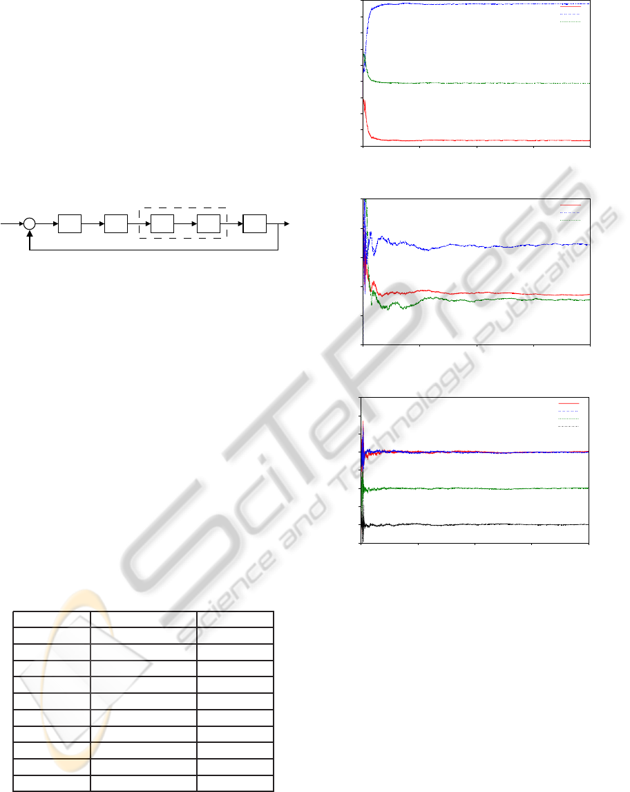
The block diagram for the estimation process can
be seen in Figure 7. Block E represents the genera-
tor of excitation signal PRS, NL block represents the
dead-zone nonlinearity, blocks A and T are respec-
tively the dynamics of the valve and tank and repre-
sent the linear part of the Hammerstein model. The
RIV estimation method with the presence of the for-
getting factor is represented by block M.
NL A T
Valve
E
M
u x y
b
θ
Figure 7: Block diagram of the level system estimation.
ESTIMATION AND COMPENSATION OF DEAD-ZONE INHERENT TO THE ACTUATORS OF INDUSTRIAL
PROCESSES
67
The block diagram of the compensation is shown
in Figure 8. Block C represents a PI controller, which
was tuned empirically so that, for the level system
without the presence of nonlinearities, the plant re-
sponse would behave without a large overshoot and
with no regime error (less than 2%). Mathemati-
cal manipulations were made so that a control sig-
nal equals to zero would correspond to a level of
50%. Block INL represents the inverse nonlinearity,
and was allocated before its respective nonlinearity.
The others blocks have the same meanings described
above.
NL TC INL A
u x yu
c
−
r
+
e
Valve
Figure 8: Block diagram of the level system with nonlinear-
ity compensation.
The dead-zone in the actuator of this process was
built with the following parameters: m
r
= 3, m
l
= 3,
b
r
= 1 and b
l
= −1. The graphics containing the
parameters estimation results of linear dynamics and
dead-zone can be seen in Figure 9. The parameter
values obtained at the end of the recursive estimation
process are shown in Table 1. The actual values of
each one are also in Table 1 for comparison.
Analyzing the estimation graphics, it is observed
that all the parameters have converged up to 7500s,
the last ones being the coefficients of the polyno-
mial B(q). The values obtained in the estimation pro-
cess are shown in Table 1, and have small errors (the
biggest errors are in the order of 10
−2
) in relation to
the real values. The algorithm showed good conver-
gence for the noise presence.
Table 1: Parameters of level system with dead-zone.
Parameters Estimated Value Real Value
a
1
-2.3271 -2.328
a
2
1.8968 1.899
a
3
-0.55309 -0.5543
b
0
0.00718 0.00713
b
1
0.02424 0.02441
b
2
0.00542 0.0053
m
r
3.0256 3
m
l
2.993 3
b
r
1.0214 1
b
l
-0.99561 -1
The controller was empirically tuned to k
p
= 0.5
and k
i
= 0.7. Figure 10 contains the graphics of plant
level output for the linear case, that is, without the
presence of dead-zone. Figures 11 and 12 represent,
−2.50
−2.00
−1.50
−1.00
−0.50
0.00
0.50
1.00
1.50
2.00
0 5000 10000 15000 20000
Time (s)
a
1
a
2
a
3
(a) Polynomial A(q).
−0.01
0.00
0.01
0.02
0.03
0.04
0 5000 10000 15000 20000
Time (s)
b
0
b
1
b
2
(b) Polynomial B(q).
−2.00
−1.00
0.00
1.00
2.00
3.00
4.00
5.00
6.00
0 5000 10000 15000 20000
Time (s)
m
r
m
l
c
r
c
l
(c) Dead-zone.
Figure 9: Parameter estimation of level system with dead-
zone.
respectively, the cases of plant output with the pres-
ence of dead-zone with and without the compensator
block. The control signals for these last two cases are
shown in Figure 13.
For track 1, the control without compensation was
rather oscillatory during the existence of the distur-
bance (10 to 40s) with the tank level ranging approx-
imately from 45 to 55%. After the disturbance, the
level returned to the reference and remained without
oscillations. This was due to mathematical manipula-
tions that keep the reservoir level by 50% for a valve
input signal equal to zero. In tracks 2 and 3 the refer-
ence is changed respectively to 49 and 51%. In these
two tracks, it is observed the existence of oscillations
ICINCO 2010 - 7th International Conference on Informatics in Control, Automation and Robotics
68
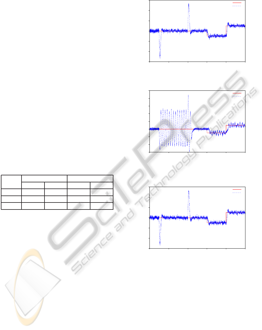
maintained in the output with amplitude around the
reference of ±1%. As for the control with compen-
sation, the behavior of the plant output is very similar
to the case where there is not the dead-zone presence.
Thereby, and according to Table 2, the control with
compensation had better IAE indices (ε
2
) for the 3
tracks compared to the control without compensation.
Table 2 also shows the index ε
1
of control signal
variance evaluation for the two cases with the pres-
ence of dead-zone. Note that, in the case with com-
pensation, the inversenonlinearity (INL block) output
was considered as controlsignal, and not the output of
PI controller. Based on the graphic of Figure 13, the
control signal with the inverse nonlinearity is more
aggressive in relation to the sign of pure PI control
for the dead-zone region. This is caused by the dis-
continuity present in the graphic of the inverse dead-
zone (see Figure 5) around de zero point. Whenever
the PI output inverts its sign (from positive to nega-
tive or vice versa), a jump in the output compensation
occurs. Even with this discontinuity, the control with
compensation had a smaller variance in its signal to
the 3 tracks of the evaluation.
Table 2: Metrics for performance evaluation of nonlinear
system with and without compensation.
Track
With Comp. Without Comp.
ε
1
ε
2
ε
1
ε
2
1 3.0574 1.7683 2.4786 0.3696
2 0.1242 0.3722 0.0492 0.2028
3 0.1201 0.4188 0.0547 0.2439
6 CONCLUSIONS
In this work, it was developed a method of estima-
tion and compensation of dead-zone that is present in
the actuators of various industrial processes. It was
used, as a testing process, a simulation of a level tank,
which has a valve with a dead-zone to control the in-
put flow.
First it was developed an estimation method of
parameters for a Hammerstein model, in which the
nonlinear part is represented by dead-zone. As linear
dynamic, the Output Error model was used, which is
a more complex model and the estimation task be-
comes more difficult when compared to the estima-
tion of ARX and ARMAX models, because the noise
is much more influential in the process. The method
used the key term separation principle, reducing the
number of parameters to be estimated.
In practice, the process operator defines the dura-
tion and type of measures that can be collected from
44.00
46.00
48.00
50.00
52.00
54.00
56.00
0 20 40 60 80 100
Level (%)
Time (s)
Reference
Output without dead−zone
Figure 10: Plant output without dead-zone.
44.00
46.00
48.00
50.00
52.00
54.00
56.00
58.00
60.00
0 20 40 60 80 100
Level (%)
Time (s)
Reference
Output without compensation
Figure 11: Plant output with dead-zone and without com-
pensation.
44.00
46.00
48.00
50.00
52.00
54.00
56.00
0 20 40 60 80 100
Level (%)
Time (s)
Reference
Output with compensation
Figure 12: Plant output with dead-zone and with compen-
sation.
the process. In fact, large variations in the excitation
signal are very useful in identifying systems. How-
ever, they are not often allowed by the operators.
Then, the identification should be made using normal
operation data.
After being estimated, the parameters that make
up the dead-zone were used to construct the inverse
model of compensation. In general, the controller
with compensation was more aggressive than the con-
trol without compensation during the dead-zone re-
gion. However, the plant output is much less oscil-
lating in the compensated case. Performance metrics
ESTIMATION AND COMPENSATION OF DEAD-ZONE INHERENT TO THE ACTUATORS OF INDUSTRIAL
PROCESSES
69

−5.00
−4.00
−3.00
−2.00
−1.00
0.00
1.00
2.00
3.00
4.00
5.00
0 20 40 60 80 100
Time (s)
Control without compensation
Control with compensation
Figure 13: Control signals for the nonlinear system.
quantify the control actions and the error at the plant
response. Therefore, the purpose of minimizing or
even canceling the oscillations was achieved.
The estimation and compensation techniques de-
veloped here can be applied to any industrial plant
that is represented according to Hammerstein model,
which has the dead-zone as nonlinearity.
It is intended, as future work, to estimate and com-
pensate the backlash nonlinearity. In addition, we in-
tend to implement the proposal in a Programmable
Logic Controller (PLC). This will bring this work to
a possible application in the real world.
ACKNOWLEDGEMENTS
Especial thanks for ANP PRH-14, CNPq and Petro-
bras.
REFERENCES
Aguirre, L. A. (2007). Introdução à Identificação de Sis-
temas: Técnicas Lineares e Não-Lineares Aplicadas a
Sistemas Reais. Editora UFMG, 3 edition.
Campos, M. C. M. M. and Teixeira, H. C. G. (2007). Con-
troles Típicos de Equipamentos e Processos Industri-
ais. Editora Edgar Blücher.
Chen, H.-W. (1995). Modeling and identification of paral-
lel nonlinear systems: structural classification and pa-
rameter estimation methods. Proceedings of the IEEE,
83(1):39–66.
Desborough, L. and Miller, R. (2002). Increasing customer
value of industrial control performance monitoring -
honeywell’s experience. In AIChE Symposium Series
2001, number 326, pages 172–192, Arizona.
FISCHER (2005). Control Valve Handbook. Emerson Pro-
cess Management, Iowa, USA.
Goodhart, S. G., Burnham, K. J., and James, D. J. G. (1991).
A bilinear self-tuning controller for industrial heating
plant. IEEE Conference Publication, 2(332):779–783.
Ikonen, E. and Najim, K. (2002). Advanced Process Identi-
fication and Control. Marcel Dekker, New York.
Ljung, L. (1987). System Identification: Theory for the
User. Prentice-Hall.
Nelles, O. (2000). Nonlinear System Identification.
Springer, Berlin.
Ulaganathan, N. and Rengaswamy, R. (2008). Blind identi-
fication of stiction in nonlinear process control loops.
In American Control Conference, pages 3380–3384.
Vörös, J. (1995). Identification of nonlinear dynamic sys-
tems using extended hammerstein and wiener mod-
els. Control Theory and Advanced Technology,
10(4):1203–1212.
Vörös, J. (1997). Parameter identification of discontinuos
hammerstein systems. Automatica, 33(6):1141–1146.
Vörös, J. (2003). Recursive identification of hammerstein
systems with discontinuous nonlinearities containing
dead-zones. IEEE Transactions on Automic Control,
48(12):2203–2206.
Vörös, J. (2006). Recursive identification of hammerstein
systems with polynomial nonlinearities. Journal of
Electrical Engineering, 57(1):42–46.
Wigren, T. (1993). Recursive prediction error identifica-
tion using the nonlinear wiener model. Automatica,
29(4):1011–1025.
ICINCO 2010 - 7th International Conference on Informatics in Control, Automation and Robotics
70
