
NONLINEAR CONSTRAINED PREDICTIVE CONTROL OF
EXOTHERMIC REACTOR
Joanna Ziętkiewicz
Institute of Control and Information Engineering, Poznan University of Technology, Piotrowo 3A, Poznan, Poland
Keywords: Predictive Control, Feedback Linearization, LQ Control.
Abstract: Predictive method which allows applying constraints in the process of designing control system has wide
practical significance. The method developed in the article consists of feedback linearization and linear
quadratic control applied to obtained linear system. Employment of interpolation method introduces
constraints of variables into control system design. The control algorithm was designed for a model of
exothermic reactor, results illustrate its operation in comparison with PI control.
1 INTRODUCTION
The predictive algorithms have a wide industrial
applications because of the simplicity of its
operation and good features of regulation. One of
important advantages of the predictive control is the
possibility to impose the signal constraints in the
process of designing the control law. In the practical
applications it is convenient to use the linear models
for the theory of them is well known.
First examples of the industrial use of the MPC
applications had place in 1970’s, but the idea was
known earlier (Lee, Markus, 1967). One of the most
important algorithms was the Dynamic Matrix
Control (Cutler, Ramaker,1980) and Quadratic DMC
(Garcia et al.,1989) with linear models. There
appeared a number of articles with nonlinear models
with the exact and suboptimal algorithms. The use of
nonlinear models cause additional problems with
finding global minimum and can have an effect on
calculation time (Tatjewski, 2002). Adaptation of a
controller with linearization around the working
point may result in system instability (Dimitar et al.,
1991), changes of variables have to be limited.
The aim of the work was to design an application
used for control of an exothermic reactor with
constraints, to propose use of feedback linearization
for this nonlinear plant, present predictive control
method solving problem of constraints(Poulsen et
al., 2001) and its modification (Ziętkiewicz 2008)
for changed reference signal.
2 EXOTHERMIC REACTOR
2.1 CSTR Model
The plant to be controlled is the Continuous Stirred
Tank Reactor (CSTR). The structure of reactor is
presented on figure 1. It contains tank, cooling
jacket, inflow and outflow of both elements. It is
assumed that, because of perfect mixing, there are
no spatial gradients of parameters in the tank area.
The work of reactor is described by 3 differential
equations. First equation (1) illustrates the mass
balance,
),()(
)(
tVRtCC
dt
tdC
V
i
(1)
where C(t) is the concentration of product measured
in [kmol/m
3
]. The second and the third equations
(2,3) represent the balance of energy in the reactor,
T,C
T
i
,C
i
T,C
T,C
Φ
j
,T
j0
T
j
Φ
Figure 1: Model of exothermic reactor.
),()()()(
)(
tVRtQtTTc
dt
tdT
cV
iipp
(2)
208
Zi˛etkiewicz J. (2010).
NONLINEAR CONSTRAINED PREDICTIVE CONTROL OF EXOTHERMIC REACTOR.
In Proceedings of the 7th International Conference on Informatics in Control, Automation and Robotics, pages 208-212
DOI: 10.5220/0002954202080212
Copyright
c
SciTePress

and the balance of energy in the cooling jacket
0
()
() () ()
j
j j pj j j pj j j
dT t
vc tcT Tt Qt
dt
(3)
where T(t) is the temperature inside the reactor and
T
j
(t) temperature in the cooling jacket, measured in
Kelvin.
)(t
j
[m
3
/h] represents cooling flow through
the reactor jacket. Remaining equations represent
)()()( tTtTAtQ
jc
(4)
- thermal energy in the process of cooling,
()
0
() ()
E
R
Tt
Rt Ctke
- velocity of reaction.
(5)
Constant values used in experiments are placed in
the table 1.
Table 1: Constant values of CSTR model.
const. value const. value
1.13 [m
3
/h] T
j0
294.4 [K]
V 1.36 [m
3
] ρ
j
998 [kg/m
3
]
C
i
8 [kmol/m
3
] c
pj
4186.8 [J/(kgK)]
ρ 801 [kg/m
3
] k
0
7.08*10
10
[1/h]
c
p
3140.1 [J/(kgK)] E 6.96*10
7
[J/kmol]
T
i
294.4 [K] R 8314.3 [J/(kmolK)]
(-Δ
i
) 6.96*10
7
[J/kmol] α
c
3.07*10
6
[J/(hKm
2
)]
v
j
0.109 [m
3
] A
c
23.2 [m
2
]
In the further parts of the paper the function of
time will be omitted to simplify equations. The
control signal will be denoted as
)(tu
j
and the
state variables x
1
=C(t), x
2
=T(t), x
3
=T
j
(t). The system
(1-3) can be describe by 3 equations:
2
2
/
11 10 1
/
21 11213 10
03
3223
(),
() ,
() ,
ERx
i
E
Rx
i
j
j
xAC Ake x
xATABxBxCxke
Tx
xBxx u
v
(6)
where
,
1
V
A
,
1
p
cc
cV
A
B
,
2
pjjj
cc
cv
A
B
.
)(
p
i
c
C
2.2 Formulation of Control Problem
The objective of control is to make the temperature
inside the reactor T(t) track a desired trajectory w(t)
using the control signal u. The complete model with
output signal can be described by (6) with defined
output signal
.
2
xy
(7)
Furthermore the control signal is constrained
hmhm
j
/5.2/0
33
(8)
3 FEEDBACK LINEARIZATION
The functions describing the considered system are
smooth and have continuous derivatives of any
required order in region Ω={(x
1
, x
2
, x
3
)єR
2
|x
2
>T
j0
,
x
3
>T
j0
}, which is the normal area of reactor
operation. Since the relative degree is equal to 2 and
the system order was equal to 3, the system has
internal dynamic described by one equation. From
(6) it takes form:
.)(
1
/
0111
xekACAx
RyE
i
(9)
Parameters E and R are positive (tab.1). The output
signal y is also positive. If we assume, that control
law provides, that signal y is bounded
(y(t)=e(t)+w(t), where e(t) is the tracking error), then
the internal dynamic of the system is stable.
The system (6,7) can be described in a the form
).(
)()(
x
xxx
hy
ugf
(10)
There exists a diffeomorphism z=φ(x) in region
Ω,
)(
)(
)(
)(
3
2
1
x
xhL
xh
z
z
z
f
x
(11)
which conditions normal form of transformed
system. L
f
h(x) is the Lie derivative of h(x) with
respect to f(x). All variables of vector z have to be
independent, therefore η(x) should satisfy L
g
η(x)=0.
One of solutions is η(x)=x
1
. The feedback law is
defined as
,
)(
)(
),(
2
x
x
x
hLL
hLv
vu
fg
f
(12)
where v is the new input signal. The feedback
linearization method is illustrated in fig.3.
The system with new coordinates takes form
,
)(
3
/
011
2
3
2
1
1
zekACA
v
z
z
z
z
RzE
i
(13)
1
zy
,
for which the mapping z=φ(x):
(14)
NONLINEAR CONSTRAINED PREDICTIVE CONTROL OF EXOTHERMIC REACTOR
209

,)()(
1
/
013121111
2
2
x
ekCxxBxBATA
x
RxE
x
(15)
and the inverse mapping x=φ
-1
(z):
1
3
1
1
/
1112 30 11
1
() .
()
ERz
z
z
ABzz Czke AT
B
z
The transformed system is linearized partly, the third
equation is nonlinear. However, the relation between
input and output signal is linear, which will be used
in control algorithm.
nonlinear
v
(
t
)
Ψ(
v
,
x
)
x(t)
φ(
x
)
u(t)
z(
t
)
y(t)
Figure 2: Feedback linearization.
4 PREDICTIVE CONTROL
To design the control algorithm we will use linear
model obtained in previous section
.
1
2
2
1
zy
v
z
z
z
(16)
Third equation of (13) will be used only to calculate
successive variables of vector z, and then from (15)
vector x. After discretisation of the linear model
with T
s
=60s and adding reference signal w
k
which is
imposed by using an additional variable
,
1 kkkk
ywpp
(17)
we obtain a discrete model
,0
,
1
0
0
1
0
1
k
dk
kk
d
k
d
d
k
p
z
Cy
wv
B
p
z
C
A
p
z
(18)
where A
d
, B
d
, and C
d
denote matrices of discrete
model.
4.1 Linear Quadratic Control
The predictive control algorithm for the system
without constraints and infinite horizon can be
designed by LQ control method (Maciejowski,
2002). The cost function which prevents too large
deviation from equilibrium point is given by:
00
02
00
(),
T
kk kk
tkk
kt
kk kk
zz zz
JQRvv
pp pp
(19)
with
100
010
001
Q
and R=0.1. The optimal gain L is
obtained from LQ method. Then the control law
describes
,
ˆ
ˆ
ˆ
|
|
tk
ttk
p
z
LMwu
(20)
where M is the first element of L, because the output
is the first element of the state vector z. The index k|t
denotes the sample of variable predicted for the
moment t and calculate in the instant k.
4.2 Constrained Predictive Control
In order to include the constraints to the control
problem, there will be applied the interpolation
technique (Poulsen et al., 2001). It consists in using
the LQ method for a system with so changed
required output trajectory
tk
w
|
~
that the obtained
variables fulfil the constraints. The changed
trajectory is defined by
,
ˆ
~
|| tkttk
sww
(21)
then the control law
.
ˆ
~
ˆ
||| tktktk
zLwMv
(22)
The so called perturbation trajectory
tk
s
|
ˆ
calculated
in the instant k for successive steps k≤t≤H is
obtained from
tkktk
ss
|1|
ˆˆ
,
(23)
where 0≤α
k
≤1.
It can be seen from (21) and (23), that α
k
=0
corresponds to the unconstrained LQ control. To
find proper
tk
s
|
ˆ
assuring feasibility of
tk
w
|
~
we use
the initial perturbation trajectory
t
s
|0
ˆ
, which ensures
fulfilling the constraints. One of solution is to chose
the
t
s
|0
ˆ
so it maintains trajectory
tk
w
|
~
unchanged for
future t, therefore every variable in model is
unchanged (assuming that initial condition is stable
and fulfil given constraints).
ICINCO 2010 - 7th International Conference on Informatics in Control, Automation and Robotics
210
With above reasoning the objective of control is
to minimize the parameter α
k
with respect to
constraints on assumed horizon H. Even though the
model (18) is linear, the relation between
constrained variable u and α is nonlinear, because it
goes through the function
),( xvu
. To solve this
nonlinear problem it is possible to use simple
numeric procedure as bisection.
The above procedure was designed for the
instant change of the set point. When desired output
trajectory w
k
changes in another way the following
method of calculation of
tk
s
|
ˆ
can be used:
tkktktktk
swws
|1|1||
ˆˆ
.
(24)
Under assumption that initial conditions are
stable and then the initial perturbations sequence is
stable, because of the constraints values the control
law designed on the interpolation algorithm is
asymptotically stable.
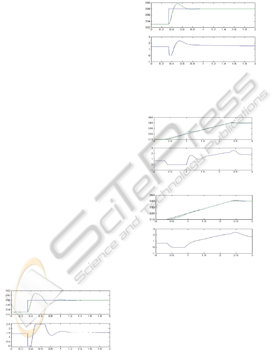
5 RESULTS
Two experiments were performed in matlab
environment. The PI controller tuned experimentally
was used as comparison was. In the first experiment
the trajectory w
t
was suddenly changed from one
value to another. In the second experiment w
t
was
changed along the linear function, which is a proper
behaviour of desired temperature in the reactor. In
every figures placed below first chart illustrate the
desired trajectory w
t
and the output y
t
, whilst the
second chart show the behaviour of constrained
input of the reactor u
t
.
The results of the first experiment are illustrated
below. The desired trajectory was changed from 333
to 338K with jump in t=20min. Figure 4 illustrate
the result obtained from use of PI method, figure 5
with predictive algorithm developed in the article.
t[h]
u
t
[m
3
/h]
t[h]
Figure 3: First experiment, PI control.
w
t
,y
t
[
K
]
t[h]
u
t
[m
3
/h]
t[h]
Figure 4: First experiment, predictive control.
In the second experiment trajectory was changed
in linear function from 310 to 340K. Results are
placed below in a way as in the first experiment.
Figure 5: Second experiment, PI control.
Figure 6: Second experiment, predictive control.
5.1 Conclusions
The operation of predictive method presented in the
paper was correct, it fulfils the constraints. In both
experiments the use of the algorithm improved the
quality of control in comparison with PI control.
However the disadvantage of the method is that it
relies on feedback linearization, which can be use to
limited class of objects.
REFERENCES
Cutler C. R., Ramaker B. L., 1980. Dynamic Matrix Con-
w
t
,y
t
[K]
w
t
,y
t
[K]
u
t
[m
3
/h]
t[h]
t[h]
w
t
,y
t
[K]
u
t
[m
3
/h]
t[h]
t[h]
NONLINEAR CONSTRAINED PREDICTIVE CONTROL OF EXOTHERMIC REACTOR
211

trol – a computer control algorithm, in Proc. of Joint
Automatic Control Conference, San Francisco.
Dimitar R., Ogonowski Z., Damert K., 1991. Predictive
control of a nonlinear open-loop unstable
polymerization reactor, in Chemical Engineering
Science, 46, 2679-2689.
Garcia C. E., Prett D. M., Morari M., 1989. Model
Predictive control: theory and practice – a survey, in
Automatica, 25:335-348.
Lee E. B., Markus L., 1967. Foundations of Optimal
Control Theory, J. Wiley, New York.
Maciejowski J. M., 2002 Predictive Control with
constraints, Prentice Hall, Pearson Education Limited,
Harlow, UK.
Poulsen N. K., Kouvaritakis B., Cannon M., 2001.
Constrained predictive control and its application to a
coupled-tanks apparatus, in International Journal of
Control, Vol.74, 552-564.
Tatjewski P., 2002 Sterowanie zaawansowane obiektów
przemysłowych, Exit, Warszawa.
Ziętkiewicz J., 2008. Sterowanie predykcyjne z
ograniczeniami dla modelu egzotermicznego reaktora
chemicznego, in Proc. of XVI Krajowa Konferencja
Automatyki, Szczyrk.
ICINCO 2010 - 7th International Conference on Informatics in Control, Automation and Robotics
212
