Shadow Artifacts Correction on Fine Art Reproductions

S. A. Bibikov

, V. A. Fursov

and A. V. Nikonorov

Image Processing Systems Institute of Russian Academy of Science

151, Molodogvardeyskaya, 443110 Samara, Russia

Samara State Aerospace University named after academician S. P. Korolyov

34, Moskovskoye shosse, 443086 Samara, Russia

Abstract. The paper under consideration deals with information technology for

correction of shadow artifacts on colour digital images obtained by taking

photos of paintings with the purpose of their reproduction. Appearance of

shadow artefacts is caused by different intensity of picture lighting. The

problem of shadow detection and subsequent colour correction in this area is

solved.

1 Introduction

Digital images of paintings are used to create the reproductions of pictures, virtual

museums, and digital catalogues of paintings preserved in the museums. Usually, they

are obtained by one of two ways: either by direct recording into the digital camera, or

by scanning the negative images and slides made before. When taking a photo of a

picture, the main problem is to provide a uniform intense lighting of the entire picture

surface. For this purpose, the painting is lighted from both sides by floodlight

projectors. Thereby, due to different remoteness of illuminators, shadow stripes are

appearing along the edges of the frame.

Paper [1] deals with the task of removing the shadow using two images of the

same subject, one of which has been obtained in the natural environment, and the

other by means of additional lighting (i.e., flashlight). The problems of color

reproduction and correction of color artifacts on digital images were also solved in

papers [2-7], [14].

In these papers, cases of uniform shadowing along the image area were

investigated.

In this paper, we consider an information technology for removing the shadow in a

situation, when the single unique copy of painting is available, and the shadows are

located in some area. The paper deals with correction methods based on applying an

algorithm for histogram transformation and identification of formal transformation

model of lightness function.

A. Bibikov S., A. Fursov V. and V. Nikonorov A. (2010).

Shadow Artifacts Correction on Fine Art Reproductions.

In Proceedings of the Third International Workshop on Image Mining Theory and Applications, pages 3-12

DOI: 10.5220/0002959800030012

 SciTePress

2 Problem Definition

The registration of fine art image is suggested to be implemented in such a way, that

the axes of coordinates connected with the sides of a rectangular picture frame and

digital image are parallel.

For definiteness, let us suppose that a system of coordinates begins at the left

lower corner of a rectangular picture frame, the OY-axis is directed upwards, and the

OX-axis directed to the right. Axes oy and ox of the rectangular window of

registration device are directed accordingly, and deviations of these axes OY,

oy and

OX , ox from parallelism may be neglected.

In the present paper, we limit our consideration to removing a shadow stripe along

the left lateral side of image, so that the left boundary of stripe coincides with the OY-

axis. One can easily note that the algorithms for removing the shadow stripe located

along any boundary of image will not change, if system of coordinates will be rotated

accordingly.

Usually, the lighting equipment does not cause any perceptible color distortion.

That is why in the present paper, to detect and remove the shadow distortion, we only

use information about lightness of pixels. It is known [8] that the information is

contained in the lightness components of some color spaces. Specifically, the CIE Lab

color space is used in the present work.

In case when the lighting equipment causes any additional color distortion,

correction is also to be performed in channels carrying the information about color.As

these distortions are distributed uniformly along the image field, the task can be

solved after removing the shadows by methods considered in papers [2-7].

Let us give the definition of a shadow. Let k be a number of row parallel to ox -

axis and reckoned in the direction of

oy -axis. Consider an interval





0, N in this row.

Let





be some point within the interval. Assume that for the k-th row of the

uniformly illuminated image, the equality of means within the intervals left and right

from this point is valid:

 

ki ki

Lx Lx

sNs











(1)

where



Lx are values of lightness at the

-th points of the k-th image row.

As a shadow on the interval











we shall call a distortion, whereby for any

interval

,0,







holds the following inequality

 

ki ki

is is

Lx Lx d

 



















(2)

where d is a parameter characterizing the shadow intensity. Here and elsewhere, the

values of lightness, in case of the illuminated dots of image, are designated as





and in case of the shaded dots as







Due to the fact that the light source is not a point source, the shadow boundary, as

a rule, proves to be fuzzy.In this case, the definition of shadow (1) and (2) still holds,

if the diffusion function is smooth and has no ridge point (sign reversals of the

derivative). In this case, as a frontier point



of shadow field we take a point, where

the diffusion function is equal to half-sum of its extreme values. From now on this

point will be called middle point of twilight area. Thus, the locus of



is a boundary

shadowed area. Examples of the



locus are shown on fig. 3.

Furthermore, the shadow field for various rows k may differ because of the relief

of picture frame. Thus, the shadow field has two regions, the distortion character of

which and, consequently, the methods for their correction must differ, and the

boundaries of these regions are in general not rectilinear.

Directly to the

OY -axis adjoins the (main) area with the uniform shading, the

latter being determined by the parameter d. Between this area and illuminated area

there is a twilight area, generally more narrow, which shading is decreasing towards

the

OX -axis. The boundaries of the twilight area separating it from the shaded and

illuminated fields are curved. Usually, the X-coordinate of these curves has a slight

spread with respect to a straight line parallel to the

OY -axis.

Thus, the problem is to determine the boundaries of main and twilight area of

shadow and to elaborate the algorithms for color correction in each of these fields

taking into account the peculiarities of variations of shadow distortion intensity in

each of them. The proposed information technology is oriented at implementation in a

distributed computing system.

3 Detecting a Boundary of Shadow Area

The task of detecting the boundaries of shadow area is, in fact, the task of edge

detection [13]. The most approximate to it is the task of edge detection in the CIE Lab

color space considered in [10]. In the said paper, the so called method of active

contours [9][11] was employed based on the theory of curve evolution. But in our

case, this method can not be used in original form, as the contours of the fields are

fuzzy. In the following, we consider the algorithm for detecting the boundaries of

shadow area accounting for the mentioned peculiarities of contours.

The problem is solved in two steps. First, we determine a set G of points



yG pertaining to the so called midline of the twilight area oriented along the

oy -axis. Then, the entire twilight area is formed in its neighborhood.

Let us consider a lightness component L of a three-component color image. To

detect the boundary of shadow area introduce a criterion. For the point



, being a

boundary of the shadow field determined by Eq. (1) and (2), the so called contrast

indicator is introduced:





sCC





(3)

where



Lki

CLx

















are estimates of the mean value of lightness function within the intervals









and 1,







respectively, and N is a number of lightness values within the

investigated image area in the direction of the

ox - axis.

Thus, it will be sufficient for the point



to be the boundary of shadow area at the

k-th row, if the contrast indicator (3) is distinct from zero and assume the maximum

value at this point. Consequently, to detect the boundary of shadow field it is

necessary to compute the values of the contrast indicator (3) at every point of the row,

to choose the row where it proved to be the maximal one, and to verify that the

contrast at this point is perceptible enough. Proximity of contrast parameter values in

the neighboring rows can be an additional condition of shadow existence.

We should emphasize once more that in reality the statements (1) and (2) do not

hold exactly. But the differences between the means within the intervals are generally

much less than the contrast caused by shadow. That is why the procedure described

turns out to be effective in a wide range of shading intensity.

The following modification of indicator (3) improves the fidelity of identification

in many cases. This modification is based on calculations of two means of two

symmetrical intervals of a pixels, divided by (2b+1) pixels:

This modification is based on a calculation of mean values on two symmetrical

intervals of size a , spaced (2b+1) pixels apart:

 

(, , )

sb sab

ki ki

isab isb

sab L x L x

 

 





(4)

here a and b are parameters, requiring additional identification.

Indicator (4) is more localized then (3) and its computation is more robust to

behavior of lightness function in twilight area. If distance(2b+1) is greater then width

of twilight area, then maximum value of indicator (4) does not depend on lightness

function behavior. When b = 0 and a = N the indicator (4) acts like indicator (3), when

b = 0 and a = 1 this is like expression for first difference.

The shadow boundary point is defined by:

*( , ) max ( , , )

ab arg gsab



(5)

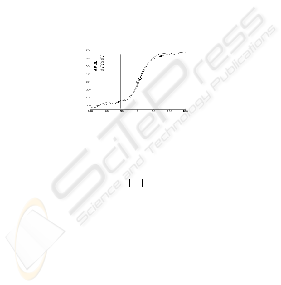
Typical values of indicator (4) and s* is shown on figures 1. and 2. On first figure

profile of lightness function L for 50-th row of image from fig 3a is shown, also on

this figure the line chart of g(s, 20, 15) is presented. On the next figure is shown the

graph for s* function for fixed value of b. Presented graphs are typical for most row

of investigated image, thus indicator g(s, 20, 15) can be used for shadow boundary

detection on this image.

0 50 100 150 200 250 300

100

120

140

160

g(s,20,15)

L(x)

0 5 10 15 20 25 30 35 40

100

120

140

160

180

Fig. 1. a) Graphs of the lightness function and of the contrast indicator for the 50-th row for

image form fig. 3 b) Graph of s*(b) dependence.

If the values



Lx are distorted by the noise (particularly, by the impulse one),

the errors of detecting the shadow boundaries in different rows may occur. To

maintain the smoothness of shadow field boundaries by the transition from





yy , the additional restriction may be imposed:

1kk dist





(6)

Here,



is a point pertaining to the midline of twilight area at





dist

 is

a variable defining the maximal admissible jump. If an initial point of midline within

the twilight area



yG is specified, subsequent applying the expression (6)

allows us to determine the sufficiently smooth shadow border (set G).

4 Detecting the Boundaries of a Twilight Area

In the course of correction on the twilight area the fact, that the width of this area is

varying at different image areas should be taken into account. This is caused by

variances of distance between different parts of the frame and the light-source. In

particular, on the edges of the frame which are more distant from the light source, the

shadow boundary is moving off from the

oy -axis and the twilight area is getting

wider. In this section, procedure of detecting the boundaries of twilight area with

regard for the said peculiarities is considered. It is based on the midline of shadow

boundary, and the method for detecting this boundary was described in the previous

section.

The idea is to approximate the lightness function within the twilight area specified

by the steady increasing function. Actual lightness functions may essentially differ

owing to superposition of shadow upon various picture elements in the rows. This is

why approximation is implemented with respect to some averaged lightness function

values obtained by summing the lightness functions of several neighboring rows.

With this purpose, the values of lightness functions in the rows are taken in such a

way that the indications of each row pertaining to the midline of shadow boundary

coincide. Let us designate a mean of lightness function values pertaining to the

midline of shadow boundary in the local subset of rows as





0w . Mean value of

lightness indications at the distance of one pixel towards the negative values of the

-axis designate as



1w  , and towards the positive values of the

-axis as





etc.

Further on, the values of lightness function for all the rows, assigned numbers of

which are equal, are averaged. As a result, for the twilight area, a set of lightness

function values averaged within the local set of rows is formed (Fig. 2):



















,..., 1 , 0 , 1 ,...,wn w w w wn

(7)

where n is selected in such a way that

max

21minSn D



 , where

max

is the

maximum possible length of twilight area within a set of all rows of the distinguished

subset, D is a distance from the point of shadow to the next image boundary.

Fig. 2. Detecting boundaries of the twilight area.. (1) is the initial function, (2) – approximating

function, (3) – point of the shadow line, (4) – amended point of the shadow line, (4-5) –

boundaries of the twilight area.

To detect the boundaries of twilight area within the allocated local area of rows,

we have to solve a problem of approximating the said set of lightness values (7) to a

function given by







bx c

wx d

ax c









(8)

Parameters c and d are introduced to estimate a shift of shadow boundary midline

within the local set of rows. The bias usually occurs due to different lightness of

picture elements within the illuminated and shaded fields.

Estimates of the parameters

,,,abcd

for each midline of local subset of rows are

made applying the least absolute values method. To make the estimates for the next

row, the last row is eliminated from the local subset and a new row is added instead.

As an initial approximation for subsequent rows, estimates of the parameters obtained

in the previous step are used.

As a result, we have a set of parameter estimates of the function (8) for each row

(except several rows from the beginning and the end). Using these estimations, the

amended mean of lightness function in each row is built. In particular, position of a

point pertaining to the midline of shadow boundary, and the values of approximated

lightness function corresponding to the shifted points are amended:

   

, , 0, 1,..., .

ixicwiwidi n  

Using the amended approximated lightness function of twilight area for each

middle of local subset of rows, the boundary values of twilight area are defined by





bor







(9)

where

is the amended coordinate of a point pertaining to the midline of shadow

boundary,







max

bor

wx w x

, and





wx

is the given admissible deviation of

lightness function from the maximal value of approximating curve at the boundary

point of twilight area.

Moreover, for each row in the neighborhood of the amended point pertaining to

the midline of shadow boundary there is a set of values of the approximated lightness

function which, in fact, are weighting factors characterizing a change of shading

intensity in the direction of

ox -axis.

5 Algorithm for Color Correction

Algorithms for color correction of shadow distortions in uniformly shaded and

twilight areas are developed by a different ways. When solving a problem in the

Lab

color space only one of them (i.e., lightness component L) is responsible for a

shadow. Thus, for shadow correction it seems reasonable to apply a popular method

for correction the lightness of grayscale images, that is, equalisaton of histogram [11].

In the course of testing a method for transformation of histograms on test and real

images, the main defect of this approach was revealed, namely, appearance of the

posterization effect, i.e. merging of different, but neighboring lightness values as a

result of transformation. In this paper, we develop an approach first proposed in [12]

and based on solving a problem of identification of formal model for color

transformation. Consider peculiarities of its applying for the present case.

Designate the coordinates of two points selected from the shaded and illuminated

image areas as



y and



y respectively. By assumption, at the absence of

shading and at uniform picture illumination, the colors of these points are similar:









ll rr

ij ij

Lxy Lxy .

(10)

In the following, the points meeting the condition (10) will be called

matching

points

. It is obvious that for an shadowed image holds the expression:









ll rr

ii i i

Lx y Lx y .

Take into consideration the transformation function





* establishing a relation

between the brightness values of matching points as follows:







ll rr

ii i i

Lx y Lx y











(11)

Having registered the lightness values for

N pairs of matching points from the

shaded and illuminated areas, the matrix relation can be written on the basis of Eq.

(11) as follows:





LLψ

(12)

Components of vector

L consist of lightness values at the matching points of the

illuminated area. Matrix

L is composed in assumption that the transformation

function (12) is a third-order polynomial. Components of vector

ξ are errors of

registration, approximating the model etc.

The sought-for estimates of transformation model parameters may be defined

using the least-square method:









*T * *T

rr rl

ψ LL LL

or by any other means (for example, using the least absolute values method).

Further on, utilizing the obtained estimate of vector of function

parameters

due to the transformation function (21), we perform a pixel-by-pixel transformation of

lightness values in the shaded field according to the expression







 

210

ˆˆˆ

,,.

ii R ii

Rii Rii

Lx y L x y

Lxy Lxy









(13)

The order of model (11) may be depressed if the estimates for coefficients of

higher orders of polynomial are found to be relative small.

The pixel-by-pixel transformation of lightness values in each row of twilight area

is performed according to the next rule:











ii ki L

Lx L x wi















ki ki

Lx Lx 





(14)

where





Lx 



is a transformation for the k-th row built in compliance with

expressions (11) – (13), and

are coordinates of the next shaded point from the

uniformly shaded area, the point being in the same row as the point under correction.

6 Results of Experiments

As test images, high-resolution digital photos of real paintings featuring a grove and

sunset were used. The images processed have the size 554

3558 and 1453933 pixels

respectively. Image format is

TIFF, color space is Lab (8 bit per channel). Enhanced

fragments of two initial images with shadow area are shown in Fig. 3a and 3c.

The image featuring a sunset is more complex in respect of detecting the shadow

boundary. Main difficulty consists in large dimensions of the twilight area (up to 120

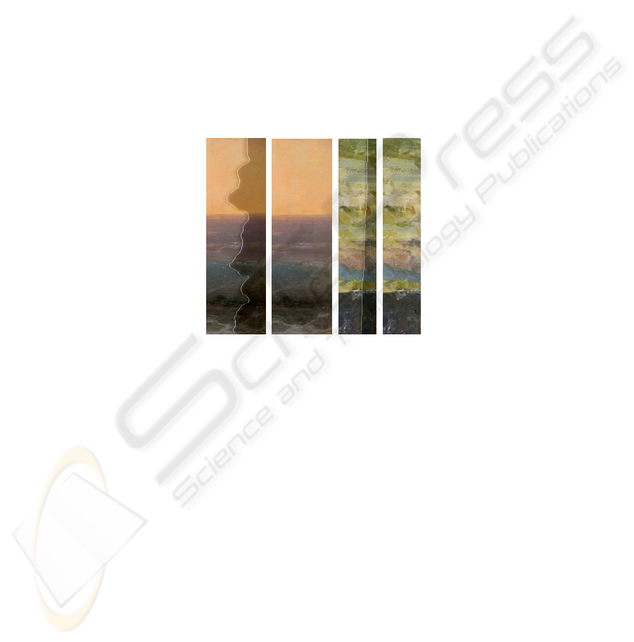
pixels). Besides, the width of this field is varying within the wide limits according to

the value of

y-coordinate.

On the image featuring a grove, the shadow boundary is rather distinct, which is

determined by small width of twilight area, whereby the boundary is almost

rectilinear. Both images feature a large number of contrast elements and are

characterized by a wide range of lightness variation in channel

L. Moreover, both

images are noisy. Said peculiarities essentially complicate identifying the weight

function (8) in the twilight areas.

Mean values within the twilight area of image featuring a sunset are represented

by a white line in Fig. 3a, c. End result after shadow artifact removing is represented

in Fig. 3b, d.

In this paper we present only two shadowed image, but our system was tested by

prepress specialists on about 200 images and demonstrates sufficient quality in 75%

cases. In other cases images needs some further correction. Altogether,

autoimmunization of shadow correction process reduce time needed for processing

one shadowed image from about one hour till 2-3 min.

Fig. 3. Example of colour correction of images with the curvilinear boundary of shadow stripe

and area of slowly changing colour: a), c) initial images with the detected shadow line; b) d)

images after correction.

7 Conclusions

The elaborated information technology for color correction of shadowed images

admits a high automation degree. Its software implementation has resulted in essential

reducing the time expenditures for prepress of color images. Apart from preparation

of painting reproductions, the technology may be employed to process the areas of

images obtained by aerospace monitoring systems and intended for print, and to

provide the services of improving the quality of digital images to a wide range of

users.

Acknowledgements

We render our thanks to the specialists of Agni Publishing House for their qualified

assistance in computer-aided color correction and testing of software on real images.

This work was supported by the Russian Foundation for Basic Research (Project

No. 09-07-00269-a).

References

1. Lu C.: Removing shadows from colorful images. PhD Thesis. Simon Fraser University

(2006).

2. Weiss, Y.: Deriving intrinsic images from image sequences. ICCV01 – IEEE V.II (2001)

68-75.

3. McCamy, C.S., Marcus H., Davidson J. G.: A color-rendition chart. J. App. Photog. In Eng

V.2. (1976) 95-99.

4. Gevers, T. Smeulders A. W. M.: Color-based object recognition. Patt. Rec. V.32 (1999)

453-464.

6. Fursov V., Nikonorov A.: Conformity estimation in color lookup tables preprocessing

problem. 7

International Conference on Pattern Recognition and Image Analisis V. I.

(2004) 213-216.

7. Nikonorov, A., Fursov, V.: Constructing the conforming estimates of non linear parameters.

4th European Congress on Computational Methods in Applied Sciences and Engineering,

Finland. (2004) 404-429.

8. Judd, D., Wyszecki G.: Color in business, science, and industry. New York: Wiley. (1975).

9. Murashev, D.M.: Automated cytological specimen image segmentation technique based on

the active contour model. Proceedings of Moscow Institute of Physics and Technology V.1,

N.1. (2009) 80-89 [in Russian].

10. Kass, M., Witkin A., Terzopoulos D.: Snakes: Active contour models. Int. J. Computer

vision, N.1 (1987) 321-331.

11. Soifer Computer V.A. et al.: Image Processing. Lightning Source Inc (2009).

12. Bibikov, S. A., Fursov V. A.: Color correction based on models identification using test

image patches. Computer optics, Samara – Moscow, Т.32 №3. (2008) 302-307 [in

Russian].

13. Furman, Ya. A., Krevetskii, A. V., Peredreev, A. K.: An Introduction to Contour Analysis:

Applications to Image and Signal Processing. Fizmatlit, Moscow. (2002) [in Russian].

14. Chuang Y-Y, Goldman, D. B., Curless B., Salesin D.H., Szeliski, R.: Shadow matting and

compositing. ACM Trans. Graph. 22 (2003) 494-500.