
Pattern Recognition Imaging for AFM Measurements
Mario D’Acunto and Ovidio Salvetti
Instituto di Scienze e Tecnologia dell’Informazione, ISTI-CNR
via Moruzzi 1, I-56124, Pisa, Italy
Abstract. The focus of this paper is on an algorithm for distortion corrections
for atomic force microscope (AFM) recorded images. AFM is a fundamental
tool for the investigation of a wide range of mechanical properties due to the
contact interaction between the AFM tip and the sample surface. When a se-
quence to AFM images correspondent to the same area are recorded, it is com-
mon to observe convolution of thermal drift with surface modifications due to
the AFM tip stresses. The surface modifications are material properties and add
knowledge to the response of the materials on nanoscale. As a consequence, a
suitable de-convolution of the thermal drifts on the recorded images need to be
developed. In this paper, we present a method for correcting thermal drifts
where the original images are corrected using a low-order polynomial mapping
function. The precision achieved and the fast computation time required make
our method particularly useful for image analysis in a wide range of applica-
tions.
1 Introduction
In the last two decades atomic force microscope (AFM) has been developed well
beyond the topographic imaging tool. It has become an important instrument for ma-
nipulation and material property characterizations at the nanometer scale. The preci-
sion of positioning has always been the key driver for AFM technology and scanning
probe microscopy in general. In an imaging tool the uncontrolled hardware drift, such
as piezo creep and thermal drift, usually causes image distortion. Some solutions
based have been proposed [1-2]. The focus of this paper is to build a method for cor-
recting the thermal drifts that represent the most important source for distortions on
sequential recorded AFM images on the same localized area. The recorded data are
divided in two classes, one is connected to topographic data, and the second one to
elastic surface Young moduli. Such two channel AFM data give the possibility to
manipulate data crossing by one class (topography) to the other one (surface elastic
map). In special way, the method for image analysis based on drift compensation is
particularly useful for time AFM sequential measurements. This last technique is used
for studying the response of viscoelastic materials to AFM tip stress. The sample used
was a low molecular weight tri-block polycaprolactone-polyethilene glycol-
polycaprolactone (PCL-PEG-PCL) copolymers. Tri-block PCL-PEG-PCL copoly-
mers present generally hard islands surrounded by soft materials. Under the stress of
an AFM tip, it has been observed that soft polymer materials can cover the hard isl-
D’Acunto M. and Salvetti O. (2010).
Pattern Recognition Imaging for AFM Measurements.
In Proceedings of the Third International Workshop on Image Mining Theory and Applications, pages 68-77
DOI: 10.5220/0002962600680077
Copyright
c
SciTePress

ands. This wearing phenomenon for viscoelastic materials does not have a clear and
exhaustive explanation due to the difficult to quantify the soft polymer coating the
hard islands. Making use of the image analysis based on drift compensation it is poss-
ible to reduce the drift in sequential AFM measurements and calculate with accuracy
the soft polymer volume moved by AFM tip. Our method is divided in two steps. In
the first one, we identify using a cross correlation function the residual thermal drift.
In the second step, we introduce a function connected to the thermal drift and a set of
specific parameter connected to low-order polynomial mapping function. The mini-
mization of such mapping function leads to the optimal parameters removing the
drifts from the sequence of the AFM images of viscoelastic sample using an useful
pattern recognition matching the images correspondent to same sample areas recorded
in different times. Our proposed method should become a powerful tool for the accu-
rate analysis of stressed viscoelastic surface and accurate quantification of AFM mul-
tichannel measurements.
2 Numerical Methods for Image-based Adaptive Drift
Compensation
The possibility of investigation of surface properties of viscoelastic materials using
AFM is based essentially on a sequence of scans on the same area to be observed.
The interpretation of data is complicated by two main factors: i), the presence of
drifts does difficult to compare AFM images acquired in different times on the same
sample location; ii), the accurate identification of specific morphological deforma-
tions of viscoelastic materials due to stressing tip resulting in a modified sequential
images with respect to the first primitive image, so leading to misinterpreted data.
Since AFM generates multiple image channels simultaneously, the spatial and tem-
poral correlation of patterns in these channels can substantially enhance the robust-
ness of the pattern detection and its position measurement, see appendix. Further-
more, the raster scanning of a probe across the same pattern back and forth embeds
asymmetric feedback control signatures for widely contact mode imaging. These
signatures provide a powerful tool to distinguish a true pattern from a set of noisy
data. Reliable pattern positioning data enable a precise adaptive control which should
achieve a sub-nanometer positioning accuracy over long period of time. The forward
scan (trace) and the reverse scan (retrace) of the same location also provide indepen-
dent information of the same patter location. In this paper, we will consider two
channels correspondent to the topographic data (first channel, quantitative data) and
surface elastic Young moduli data (second one) measured using the modulation force
AFM tool. The topographic data correspond to the height z=f(x,y) measured by the
AFM tip scanning the sample surface, see figure 5 (left). On contrary, the modulation
force channel measures in a qualitatively way the differences of surface elasticity.
Modulation force is a powerful tool for the knowledge of surface properties, never-
theless when the AFM is used for a time sequence scanning cycle on the same viscoe-
lastic sample area, it is strongly limited by its qualitatively nature.
We adopt a new method integrating a numerical corrections of thermal drifts with
pattern recognition imaging. A cross correlation function is used a priori as a method
69
for the definition of the possible range of thermal drift to be identified. There are
mainly two approaches to connect pattern recognition with location of specific fea-
tures on multi-channel images: template based method or parametric one. Template
based algorithms locate regions on the image that matche a known reference pattern.
They bare applicable when well defined and slowly changing patterns are available
on the image. Multi-channel AFM images can improve pattern location accuracy by
matching all the channels of images with their own templates, while these templates
are spatially correlated, figg. 1-2. Parametric based algorithms can be applied when
focused patterns are changing from image to image and cannot be described by image
template. These patterns, however, can be indentified by a set of measurable variables
such as geometrical and regression properties that are restricted to a certain paramete-
rized region in the space of measured variables. Parametric algorithms based on geo-
metrical patterns and spatial correlation of combined AFM images have been devel-
oped to locate the surface pattern with sub-pixel resolution in real time [2]. It is com-
monly recognized that a robust and precise drift measurement tool based on imaging
patterns is needed in order to compensate thermal drift without causing positioning
errors. Kalman filter provides the best results when dynamics of the system is accu-
rate and noise statistical parameters are fixed and known a priori. Unfortunately, this
is not generally the case for AFM measurements where both dynamics and noise
statistics may change in time and depend on viscoelastic sample, tip and environment
(humidity, temperature, etc.). In this situation, with inaccurate model and/or underes-
timated statistical parameters of the noise, Kalman filter may diverge, i.e., its estima-
tion has errors that are much greater than predicted by theory [2]. The general chal-
lenge in image analysis of AFM measurements is to provide accurate and reliable
tools to precisely locate the imaging pattern and implement real time control accord-
ing to specific applications requirements.
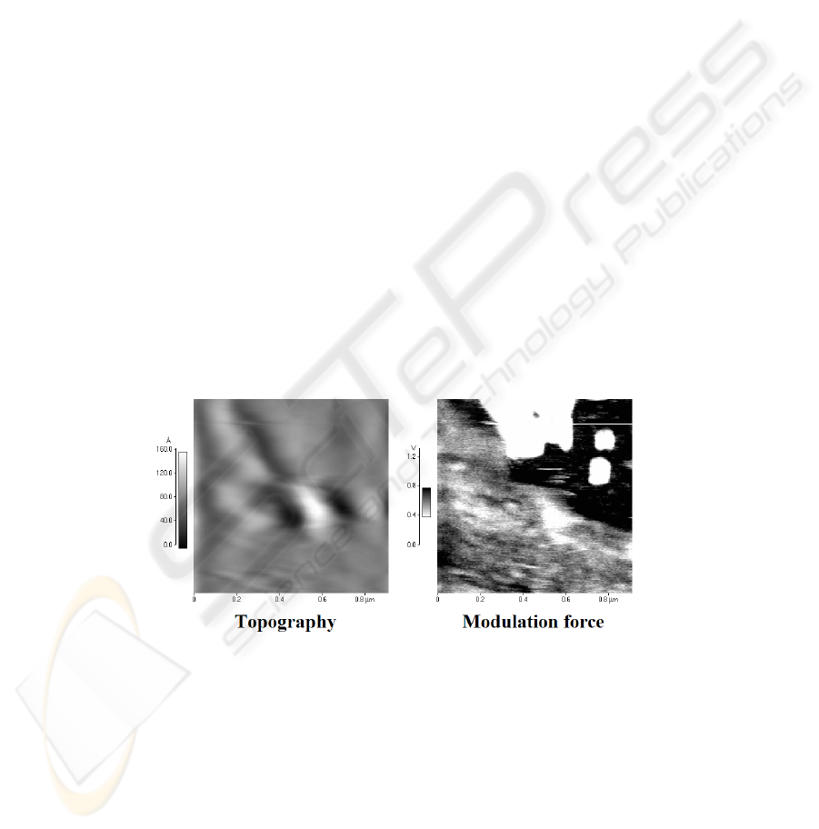
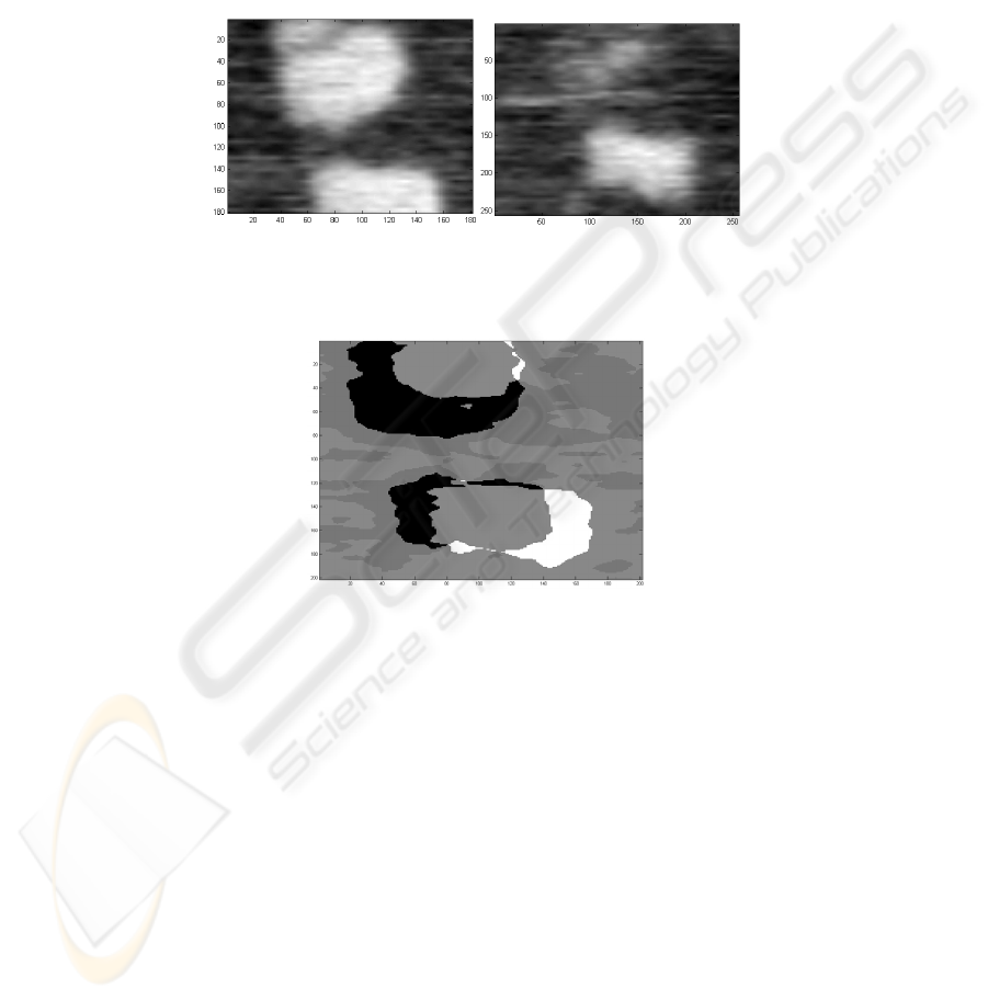
Fig. 1. A two channels AFM image of the tri-block PCL-PEG-PCL copolymer. On the contrary
to topographic data (left), the FMM image (right) shows characteristic hard domain (brighter)
surrounded by softer matrix (dark). The hard domains are approximately cylinders with the
principal axe normal to the surface. The zoom of the area surrounding the hard islands in the
Modulation force mode image are reported in the figure 2. The area considered was 1μm×1μm.
70
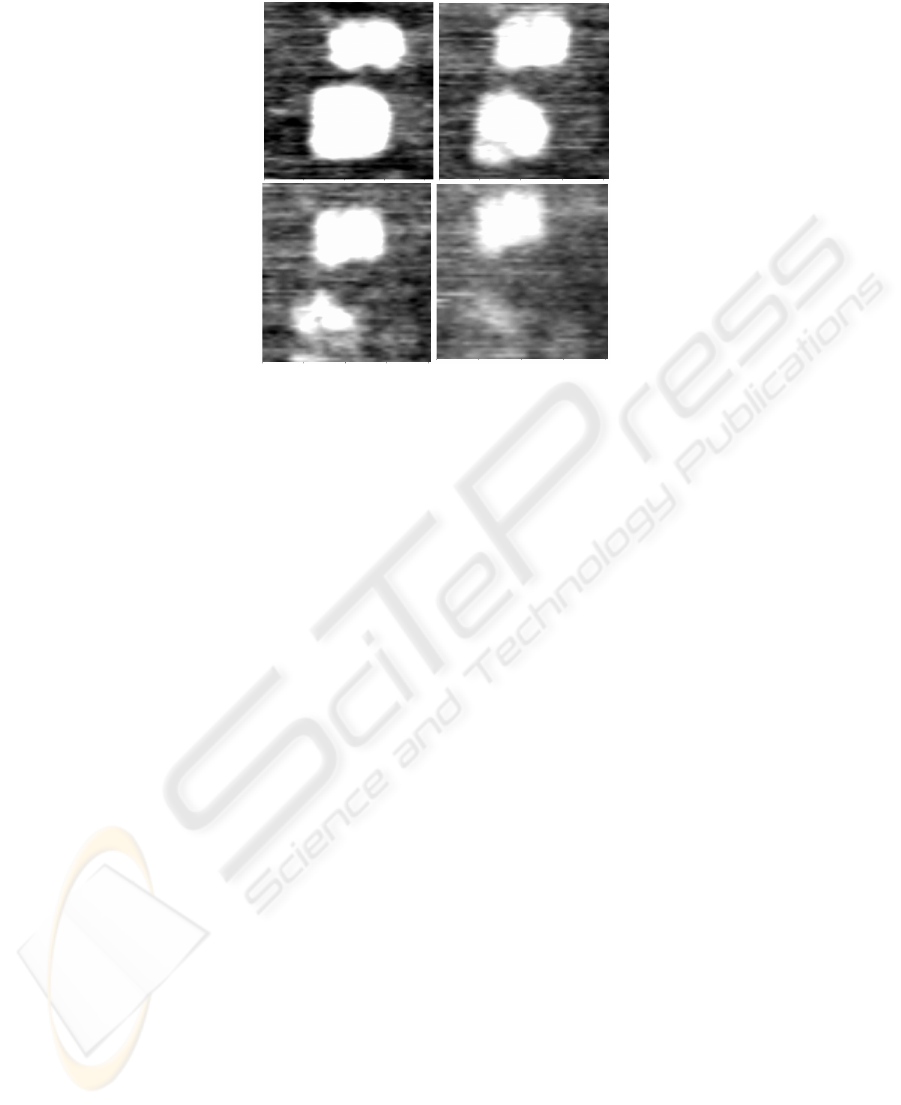
Fig. 2. Modulation Force (FMM) recorded data of 200nm×200nm areas showing two hard PU
islands (bright regions) surrounded by soft matrix (darker areas). From A-to-D: progressive
reduction of the stiff areas (white-to-grey) induced by the repeated passage of the AFM probe
tip.
2.1 A New Method for the Correction of AFM Drifts
The correction of drifts on viscoelastic AFM images is complicated by the overlap-
ping of surface effects due to tip stress that can drag polymer material from a site to
another one. As a consequence, if the displacement due to the drift, Δr, is known
during the scanning of an image, it should be possible to apply a correction based on
Δr(t) to the scanned image to recover an undistorted image. The correction can be
expressed as a mapping (x,y)→(x’,y’) between the set of points (x, y) in the image and
a new set of coordinates (x’,y’), based on the time each point was scanned. Generally,
the z-direction, i.e., the height would be not affected by relevant drifts, in special way
thermal drifts. This implies the brightness of any pixel can be considered as the “true”
value of the measurements. An other important feature of distortions is due to the
slow scanning axis. Generally, the slow scanning axis is the y-axis, while the fast
scanning axis is the x-axis. We can rewrite our mapping function (x,y)→(x’,y’) as
[3]:
)y(rxx
x
Δ
+
=
′
)y(ryy
y
Δ
+
=
′
(1)
Thermal changes is the main source for drifts on AFM image on viscoelastic ma-
terials, other distortions could arise by deformation of scanning tip or nonlinearity in
the xy stage or non-orthogonality between the x and y and z axes, can lead to position-
al errors that are functions of x and z. In our measurements, the incidence of such
distortion are not present, so we limit ourselves essentially to thermal drift. If thermal
drift is the main source drift, then changes of relative positions are not expected. If
71
the slow scanning is the y-axis, each horizontal can line may be shifted either up,
down, right, or left with respect to its neighbors, the scan line itself remains intact and
unchanged. This is because we only need to rescan a small vertical portion of the
original image and the displacement of each scan line at its center can be used as a
correction for the entire scan line.
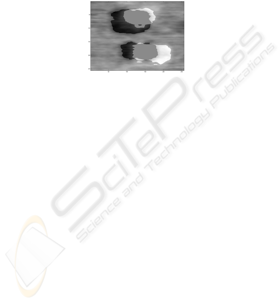
Fig. 3. Overlapping of the first and the 30-th image recorded on the same location of the vis-
coelastic sample before treatment. The shift of the hard domains could be due to thermal drift
or specific viscoelastic features due to tip stressing. Our computational methods should be able
to discriminate between the two sources of shifting. The alignments were made using a cross
correlation function, eq. (3).
Because thermal drift is a slowly varying, smooth function, we can model it as a
low order polynomial along y-direction. For moderate drift a suitable third order
polynomial could work:
3
3
2
210
yAyAyAAxx ++++=
′
3
3
2
210
yByByBByy ++++=
′
(2)
Mathematically our target is the solution of the system equations (2), i.e., to find
the set of parameters [
A
0
, A
1
,…,B
3
] which, when applied to both the original scan
yields the minimum difference between the overlapping areas of two corrected im-
ages, as in figure 3. This problem is a main topics of the broad subject of image regis-
tration, an active area of research in computer science and numerical programming
[3-5]. In comparing two images, there are two broad strategies one could pursue: i)
comparing the two images pixel by pixel; or, ii), comparing specific lists of features
that have been identified in each of the images. The first strategy has the significant
disadvantage that there are many more pixels than identifiable features, leading to
algorithms that are computationally intensive and in some sense inefficient.
The alternative strategy requires some method for identifying the appropriate fea-
tures in the images, and this raises too many problematic issues for a method to be
applicable to any scanned image. In addition some surface effect due to stressing tip
on the viscoelastic sample can produce misunderstanding features using such strate-
gy.
Following Salmons et al. [3], we adopt a strategy based on pixel-to-pixel approach
introducing a minimum difference function, defined as the minimum root-mean-
72
square (rms) difference between the pixel value of the sequence of corrected images
and the sequence of original images. The sequence of corrected images is found ap-
plying a cross correlation function. The cross correlation function for two arrays
A
and
B of discrete data points is given by [6]:
() ()( )
,. ,.,
11
N
N
j
i
x
yC AijBixjy
ji
ΓΔ Δ = +Δ +Δ
∑∑
==
(3)
where
N
i
(N
j
) is the number of data per row (column) and C is a normalization con-
stant. The position (
Δ
x,
Δ
y) of the maximum of the cross correlation function gives the
lateral shift of the images relative to each other. If the shapes of the two surfaces are
identical, the maximum lies at (0,0). To prevent the indices in the above formula from
running out of range, the performance of the cross correlation has to be restricted to a
smaller area inside the actual images leaving a border of the least the same size as the
expected image shift. Once the corrected images have been found with a cross corre-
lation function, eq. (3), we can minimize the set of parameters [
A
0
, A
1
,…B
3
], introduc-
ing the
diff-function defined as [3]:
[]
() ()
2
, ,..., , ,
01 3
11
N
N
j
i
diff function A A B z i j z i j
ts
ji
−=−
∑∑
==
⎡
⎤
⎣
⎦
(4)
where
z is the pixel value of an image at a particular point (i,j), z
t
and z
s
are the cor-
rected data image and the source (as recorded) data image, respectively. Eq. (4)
means that the mapping function (
x,y)→(x’,y’) to an area of the main image extending
beyond its own center, maximizing the area available for comparison between the two
corrected images. We have to find a global minimum of this function over the al-
lowed parameter space; in fact, there may be many local minima. A robust method is
based on using a grid search, where to evaluate the diff-function for all possible val-
ues of all eight parameters (that is, for all points an eight dimensional grid). Neverthe-
less, such method is too slow to be used on a sequence of images. In this paper we
present an alternative strategy based on an preview estimation of the most probable
couple (
Δ
x
,
Δ
y
) found as the maximum of the cross correlation function. Because the
shift is expected in the direction of the
x-direction, figure (4), we can select a strip
divided in different block numbered by
δ
. A this point the diff-function can be limited
to three only parameters:
[]
()()
2
,, , ,
1
1
ji
NN
diff function x y z i x j y z i j
ts
j
i
δδ
δ
− Δ Δ = +Δ +Δ −
∑
=
=
⎡
⎤
⎣
⎦
(5)
with the precalculation made with cross correlation function, evaluating the differ-
ence function for each new set of parameters now consists of looking-up and sum-
ming a series of array values in
diff-function[
δ
,
Δ
x,
Δ
y], one for any block
δ
. To mi-
nimize the overhead of this reevaluation, parameters lists are carefully sorted, so that
all possible parameter sets for each range of (
Δ
x,
Δ
y) are exhausted before reevaluat-
ing
diff-function[
δ
,
Δ
x,
Δ
y].
The incidence of the thermal drift is the same on both the channel AFM data, to-
pography and surface elastic moduli. We have operates the correction drift on
73

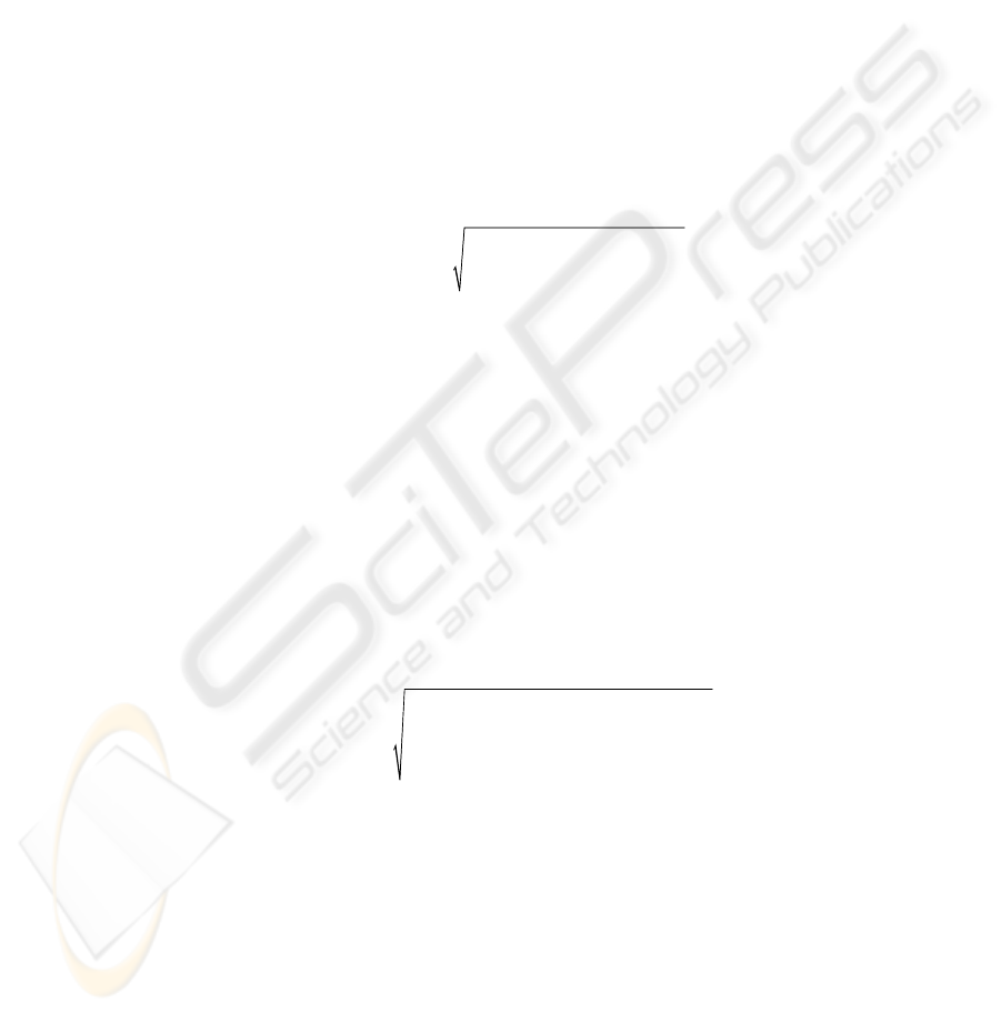
Fig. 4. Scheme showing the identification of a possible shift described by a couple (
Δ
x,
Δ
y)
identified with a cross correlation function. On right the stripe containing the possible shift due
to thermal drift along the slow scanning direction.
the modulation force data, but we can use such information on the topographic data
where pattern recognition was rather hard to do. As a consequence, after undergoing
the adjustment procedure, the new surface images correspondent to the corrected
topographic data, denoted by
A* and B*, can be compared quantitatively. We quanti-
fied the amount of volume change between the subsequent recorded data. This has
been done by integrating over the difference of the image data correspondent to the
recognized area:
() ()
**
,
*, *,
1
1
NN
ji
VBijAij
j
i
Δ= −
∑
=
=
⎡
⎤
⎣
⎦
(6)
3 Results and Discussion
The algorithm for the correction of the drift in the AFM imaging sequence was car-
ried out in two steps. In the first step, the images had to be laterally adjusted using the
cross correlation function, eq. (3). The couple (
Δ
x,
Δ
y) that maximizes the cross cor-
relation function was found [4]. In the second step, we applied the
diff-function re-
stricted to three parameters [3] to the sequence of recorded images. The application of
these two steps was justified by the fact that all the observed image shifts showed
translation movement and a small degree of rotation, figure 3, [6]. After undergoing
the adjustment procedures, the new surface images were compared quantitatively,
figures 5 and 6, and the degree of change in wear volume was calculated, figure 7.
The restricted
diff-function demonstrated to be an efficient and robust algorithm
for the minimization finding with respect to grid search. To have an idea how the
computation scales, suppose that the maximum amount of the distortion drift remains
constant ad a fraction of the image height (say, 5%), but that the number of pixels N
in the image is doubled. Maintaining single-pixel precision in the grid search requires
that the number of values of each of the parameters [
A
0
,A
1
,…,B
3
] also be doubled. For
each set of parameters, the number of blocks in y-direction to be evaluated would also
be doubled. Thus for a third order polynomial fit, the grid search should scales as
O(N
9
). Practically, downsampling an image by a factor of two should cut the time of
74
the grid search by more than a factor of 100. Subdividing an image in two and cor-
recting each half independently would have a similar impact on computation time, but
would make the method less robust to image artifacts. To have an estimation of the
computation time achieved by our method, we timed our program on a single
256
×256 pixel image, running it on a desktop computer with a single Intel Core I7
processor running a 2.93GHz. The search for the couple (
Δ
x,
Δ
y) using the cross cor-
relation function and then the minimization of the
diff-function [
δ
,
Δ
x,
Δ
y] on the
sequence of 30 images required approximately 22 s.
Fig. 5. Comparison between the first and 30-th scan after the correction of thermal drift. The
thermal drift is quantified by diff-function minimization as approximately 10nm, i.e., 5% of the
entire scanning length.
Fig. 6. This image is the equivalent of figure 3 after the correction of thermal drift using our
procedure algorithm. The overlapping of the first and the 30-th image recorded on the same
location of the viscoelastic sample present now a region of the hard island that has been coated
by the polymer. Analogously, a shift independent by thermal source is present indicating that
the hard island moved by the initial location due to reorganization of the polymer soft matrix.
If our results are confirmed by further studies and refinements of our algorithms, new insights
on the nanoscale dynamics of soft surface could be identified.
An important parameter that describes the tri-block copolymer sample surface
modifications induced by the AFM tip is the volume change between subsequent im-
ages [5]. The volume can be calculated by integrating over the difference following
the expression (6) using two subsequent acquired AFM images after adjustment. The
volume evaluation is performed on the topographic images once the drift are cor-
rected on the modulation force. The behaviour of the volume changes between subse-
quent images is shown in figure 7.
75
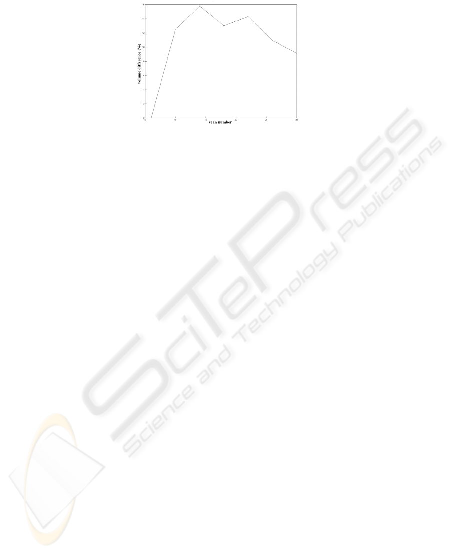
Fig. 7. Volume changes as calculated using eq. (2) between subsequent images. The volume is
calculated on topographic data correspondent to the re-aligned and computationally corrected
FMM images.
The volume variation between subsequent images presents a fast growth after an
activation barrier is reached. During the first scans the soft polymer component pre-
sents a resistance to tip induced stress. When the stress drops the activation, then the
volume percentage approaches to a sort of plateau with reduced fluctuations. It is
interesting as shoed by figure 6, that the hard islands shift position making so more
difficult for the soft component to coat the hard regions. All such results can be well
interpreted only after computational manipulation as above described. Many problem
are still open and they can be well known only after many dedicated experiments and
suitable computational algorithms. Our computational image analysis results seem go
in this direction.
4 Conclusions
The investigation of viscoelastic materials using AFM instrumentation is particularly
powerful to define the surface properties on molecular and supramolecular scale.
When a repeated sequence of AFM images on the same area, the images present a
convolution of thermal drifts and material-related modified features due to AFM tip
stressing. In this paper, we develop some algorithms for the accurate deconvolution
of thermal drift from the specific surface viscoelastic modifications. Our method
corrects the thermal drift using a low-order polynomial mapping function. The me-
thod is robust and requires short computation time, making suitable its shearing on a
wide range of applications where image analysis is required.
References
1. Yurov, V. Yu., Klimov, A. N.,: Scanning tunneling microscope calibration and reconstruc-
tion of real image: Drift and slope elimination. Rev. Sci. Instrum., 65 (1994) 1551-7
2. Clayton, G. M., Devasia, S.,: Image-based compensation of dynamic effects in scanning
tunneling microscopes. Nanotechnology 16 (2005) 809–818
76
3. Salmons, B. S., Katz, D. R., Trawick, M.L.,: Correction of distortion due to thermal drift in
scanning probe microscopy. Ultramicroscopy, available on line.
4. Gonzalez, R., Wood, R.,: Digital Image Processing. Upper Saddle River, NJ, Prentice Hall
(2008).
5. Colantonio, S., Gurevich, I. B., Salvetti, O.,: A two-step approach for automatic microscop-
ic image segmentation using fuzzy clustering and neural discrimination. Pattern Recogni-
tion and Image Analysis, 17 (2007) 428 - 437.
6. Lazzeri, L., Cascone, M.G., Narducci, P., Vitiello, N., D’Acunto, M., Giusti, P.,: Atomic
force microscopic wear characterization of biomedical polymer coatings. Tribotest, 12
(2006) 257-265.
Appendix: Background on AFM and Modulation Force Analysis
The technique for wear testing consisted in using the AFM probing tip to abrade the
surface of PU sample for approximately 30 scans while simultaneously imaging the
area where the polymer was being progressively damaged by the scanning tip.
The measurements were carried out making use of an Autoprobe CP AFM (Park
Scientific Instruments, Sunnyvale, CA) operating in contact mode. The measurements
were performed in air at room temperature and relative humidity, nearly 40%. Images
of different areas (256pixels
×256 pixels) were acquired using silicon tip (conical
shape, nominal probe radius of 10nm, nominal cantilever stiffness 0.24N/m, from PSI
manufacturer). Topographic images of square areas of 200nm
×200nm were acquired
with silicon microlevers with a spring constant of 0.24Nm
-1
, and nominal radius of
10nm. In addition to topography, mechanical properties qualitative information has
been stored making use of Force Modulation Microscopy (FMM) technique. FMM
operated in dynamic mode and allowed simultaneous acquisition of both topographic
and material-property data. It was used to detect surface elastic modulus variations on
which the image analysis was performed.
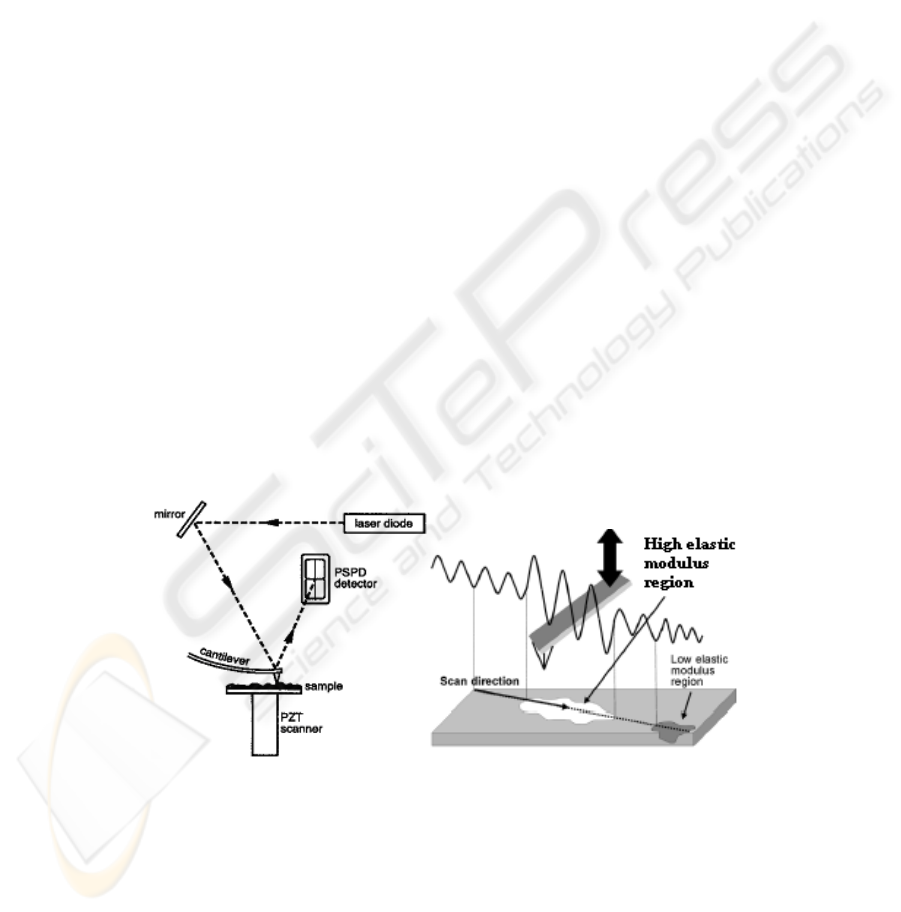
Fig. 8. On left, the schematic cartoon of an AFM. On the right, the sketch of a Force Modula-
tion Microscope (FMM). Gradients of elasticity can be record using modulation force imaging
(right) with the correspondent topography data.
77
