ANYTIME MODELS IN FUZZY CONTROL

Annamária R. Várkonyi-Kóczy, Attila Bencsik

Institute of Mechatronics, Óbuda University, Népszínház u 8, H-1081 Budapest, Hungary

Antonio Ruano

Faculty of Science & Technology, University of Algarve, Campus de Gambelas, 8005 -139 Faro, Portugal

Keywords: Power plant control, Intelligent control, Situational control, Anytime modeling, Fuzzy modeling,

SVD based complexity reduction, Time critical systems, Resource insufficiency.

Abstract: In time critical applications, anytime mode of operation offers a way to ensure continuous operation and to

cope with the possibly dynamically changing time and resource availability. Soft Computing, especially

fuzzy model based operation proved to be very advantageous in power plant control where the high

complexity, nonlinearity, and possible partial knowledge usually limit the usability of classical methods.

Higher Order Singular Value Decomposition based complexity reduction makes possible to convert

different classes of fuzzy models into anytime models, thus offering a way to combine the advantages, like

low complexity, flexibility, and robustness of fuzzy and anytime techniques. By this, a model based

anytime control methodology can be suggested which is able to keep on continuous operation using non-

exact, approximate models of the plant, thus preventing critical breakdowns in the operation. In this paper,

an anytime modeling method is suggested which makes possible to use complexity optimized fuzzy models

in control. The technique is able to filter out the redundancy of fuzzy models and can determine the near

optimal non-exact model of the plant considering the available time and resources. It also offers a way to

improve the granularity (quality) of the model by building in new information without complexity

explosion.

1 INTRODUCTION

Nowadays, solving control problems model-

integrated computing has become very popular. This

integration means that the available knowledge is

represented in a proper form and acts as an active

component of the procedure to be executed during

the operation.

For linear problems, well established methods

are available and they have been successfully

combined with adaptive techniques to provide

optimum performance.

In case of nonlinear techniques, fuzzy modeling

seems to result in a real breakthrough even when no

analytical knowledge is available about the system,

the information is uncertain or inaccurate, or when

the available mathematical form is too complex to

be used. Although, major limitation of fuzzy models

is their exponentially increasing complexity. An

especially critical situation is, when due to failures

or an alarm appearing in the modeled system, the

required reaction time is significantly shortened and

one has to make decisions before the needed and

sufficient information arrives or the processing can

be completed.

In such cases, anytime techniques can be applied

advantageously to carry on continuous operation and

to avoid critical breakdowns. Anytime systems are

able to provide short response time and are able to

maintain the information processing even in cases of

missing input data, temporary shortage of time, or

computational power (Zilberstein, 1996). The idea is

that if there is a temporal shortage of computational

power and/or there is a loss of some data, the actual

operations should be continued to maintain the

overall performance “at lower price”, i.e.,

information processing based on algorithms and/or

models of simpler complexity (and less accuracy)

should provide outputs of acceptable quality to

continue the operation of the complete system.

213

R. Várkonyi-Kóczy A., Bencsik A. and Ruano A. (2010).

ANYTIME MODELS IN FUZZY CONTROL.

In Proceedings of the 7th International Conference on Informatics in Control, Automation and Robotics, pages 213-220

DOI: 10.5220/0002966102130220

 SciTePress

There are a few approaches aiming to exploit the

advantages of anytime control however mostly in the

field of linear control. To mention two of the

characteristic approaches, Fontanelli at al. 2008

applies a hierarchical anytime control design

strategy with stochastic scheduling conditioning

resulting in usually acceptable worst-case execution

time and almost sure stability while Battacharya et

Balas 2004 uses balanced truncation and

residualization of models to generate a set of

reduced-order controllers in order to ensure smooth

switching between the truncated models.

There are mathematical tools, like Singular

Value Decomposition (SVD), which offer a

universal scope for handling the complexity problem

by anytime operations. SVD proved to be very

advantages at different fields of (linear) control, like

receding horizon control (RHC) where the

application of the technique may offer a sub-optimal

control strategy, see e.g. Rojas et al. 2004.

Embedding fuzzy models in anytime systems

extends the advantages of the Soft Computing (SC)

approach with the flexibility with respect to the

available input information and computational

power.

In this paper, we deal with the applicability of

fuzzy models in dynamically changing, complex,

time-critical, anytime systems. The analyzed models

are generated by using (Higher Order) Singular

Value Decomposition ((HO)SVD). This technique

provides a uniform frame for a family of modeling

methods and results in low (optimal or nearly

optimal) computational complexity, easy realization,

and robustness. The accuracy can also easily and

flexibly be increased, thus both complexity

reduction and the improvement of the approximation

can be implemented.

The paper is organized as follows: In Section 2

the generalized idea of anytime processing is

introduced. Section 3 summarizes the basics of

Singular Value Decomposition. Section 4 is devoted

to the SVD based complexity reduction and density

improvement of fuzzy models. Section 5 briefly

deals with anytime fuzzy control. Finally, in Section

6, conclusions are drown.

2 ANYTIME PROCESSING

In recourse, data, and time insufficient conditions,

anytime algorithms, models, and systems

(Zilberstein, 1996) can be used advantageously.

They are able to provide guaranteed response time

and are flexible with respect to the available input

data, time, and computational power. This flexibility

makes these systems able to work in changing

circumstances without critical breakdowns in the

performance. The main goal of anytime systems is to

keep on the continuous, near optimal operation

through finding a balance between the quality of the

processing and the available resources.

Iterative algorithms/models are popular tools in

anytime systems, because their complexity can

easily and flexibly be changed. These algorithms

always give some, possibly not accurate result and

more and more accurate results can be obtained, if

the calculations are continued. When the results are

needed, by simply stopping the calculations, the, in

the given circumstances best results are got.

Unfortunately, the usability of iterative

algorithms is limited. Because of this limitation, a

general technique for the application of a wide range

of other types of models/ computing methods in

anytime systems has been suggested in Várkonyi-

Kóczy, et al. 2001, however at the expense of lower

flexibility and a need for extra planning and

considerations.

3 SINGULAR VALUE

DECOMPOSITION

SVD has successfully been used to reduce the

complexity of a large family of systems based on

both classical and soft techniques (Yam, 1997). An

important advantage of the SVD complexity

reduction technique is that it offers a formal measure

to filter out the redundancy (exact reduction) and

also the weakly contributing parts (non-exact

reduction). This implies that the degree of reduction

can be chosen according to the maximum acceptable

error corresponding to the current circumstances. In

case of multi-dimensional problems, the SVD

technique can be defined in a multidimensional

matrix form, i.e. HOSVD can be applied.

The SVD based complexity reduction algorithm

is based on the decomposition of any real valued

matrix:

nnnnnnnn

ABAF

)(,2)()(,1)(

22211121

××××

(1)

where

, k=1,2 are orthogonal matrices

(

EAA

), and

is a diagonal matrix

containing the

singular values of

decreasing order. The maximum number of the

ICINCO 2010 - 7th International Conference on Informatics in Control, Automation and Robotics

214

nonzero singular values is . The

singular values indicate the significance of the

corresponding columns of

SVD

= min( , )

. The matrices can be

partitioned in the following way:

nnnk

rkk

))((, −×

nnkk

)(, ×

nnnn

))()((

)(

−×−

where r denotes “reduced” and

. If

rSVD

≤

contains only zero singular values then

and

can be dropped:

ABAF

. If

contains

nonzero singular values, as well, then the

ABAF

' =

matrix is only an approximation of

and the maximum difference between the values

and

equals

)(

1)('

iRSVD

SVD

FFE

∑

≤−=

(2)

For n-dimensional cases, HOSVD based

reduction (

)(),,,(

FHOSVDRFAA

) can

be made in n steps, in every step one dimension of

matrix

, containing the consequences is

reduced.

,...,

The first step sets

. In the followings,

is generated by step i-1. The i-th step of the

algorithm (i>1) is

1, Spreading out the n-dimensional matrix

(size: ) into a two-

dimensional matrix

nnn

i11

×× × ××

−

... ... n

n n n

in−+

* * *...* )

111

(size:

× ( *...

2, SVD based reduction of

SAABAS =≈

, where the size of

and the size of

∗

× ( nn n

in−+

*...* * *...* )

111

3, Re-stacking

∗

into the n-dimensional

matrix

1+i

(size ), and

cont. with step 1. for

nnn

i11

×× × ××

... ...

The SVD based complexity reduction can be

applied to various types of fuzzy systems, see e.g.

Takács et Várkonyi-Kóczy, 2002, and Takács et

Várkonyi-Kóczy, 2003.

4 ANYTIME MODELING:

COMPLEXITY REDUCTION

AND IMPROVING THE

APPROXIMATION

With the help of the SVD-based reduction not only

the redundancy of the rule-bases of fuzzy systems

can be removed, but further reduction can also be

obtained, considering the allowable error. This latter

can be done adaptively according to the temporal

conditions, thereby offering a way to use fuzzy

models in anytime systems.

The method also offers a way for improving the

model if later on we get into possession of new

information (approximation points) or more

resources. An algorithm can be suggested, which

finds the common minimal implementation space of

the compressed original and the new approximation

points, thus the complexity will not explode as we

include new information into the model. These two

techniques, non-exact complexity reduction and the

improvement of the approximation accuracy, ensure

that we can always cope with the temporarily

available (finite) time/resources and find the balance

between accuracy and complexity.

4.1 Reducing the Complexity of the

Model

For creating anytime models, first a practically

“accurate” fuzzy system is to be constructed. The

rule-base can be determined e.g. by using expert

knowledge. In the second step, the redundancy of

this model is reduced by (HO)SVD. The (non-exact)

anytime models can be obtained either by applying

the iterative transformation algorithm described in

Takács et Várkonyi-Kóczy, 2004 or in the general

frame of modular architecture (for details, see

Várkonyi-Kóczy et al., 2001).

In the first case, the transformation can be

performed off-line and the model evaluation can be

executed till the control action/results are needed.

The newest output corresponds to the, in the given

circumstances obtainable best results.

1+i

In the latter case, the models resulted by the

HOSVD reduction will differ in their accuracy and

complexity. An intelligent expert system, monitoring

ANYTIME MODELS IN FUZZY CONTROL

215

the actual state of the supervised system, can

adaptively determine and change for the units (rule

base models) to be applied according to the available

computing time and resources at the moment. These

considerations need additional computational

time/resources (further reducing the resources).

It is worth mentioning, that the SVD based

reduction finds the optimum, i.e., minimum number

of parameters which is needed to describe the

system.

One can find more details about the intelligent

anytime monitor and the algorithmic optimization of

the evaluations of the model-chain in Zilberstein,

1993 and Várkonyi-Kóczy et Samu, 2004.

4.2 Improving the Approximation of

the Model

The complexity of the control can be tuned both by

evaluating only a degraded model (decreasing the

granulation) and both by improving the existing

model (increasing the granulation) in the knowledge

of new information. This latter means the

improvement of the density of the approximation

points. Here a very important aim is not to let to

explode the complexity of the compressed model

when the approximation is extended with new

points. Thus, if approximation A is extended to B

with a new set of approximation points and basis,

then the question is how to transform A

to B

directly without decompressing A

, where A

and B

are the reduced forms of A and B. In the followings,

an algorithm is summarized for the complexity

compressed increase of such approximations.

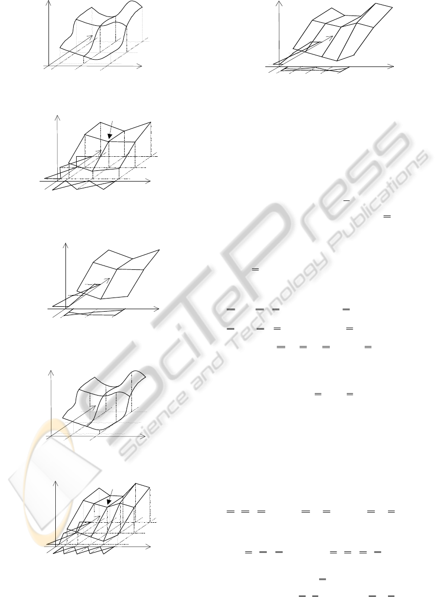
To enlighten more the problem, let us show a

simple example. Assume that we deal with the

approximation of function (see Fig. 1). For

simplicity, assume that the applied approximation A

is a bi-linear approximation based on the sampling

of over a rectangular grid (Fig. 2), so, the

bases are formed of triangular fuzzy sets (or first

order B-spline functions). After applying SVD based

reduction, the minimal dimensionality of the basis is

defined. In Fig. 3, as the minimum basis, two basis

functions are shown on each dimension instead of

the original three as depicted in Fig. 2.

),(

xxF

),(

xxF

Let us suppose that at a certain stage, further

points are sampled (Fig. 4) in order to increase the

density of the approximation points in dimension X

hence, to improve approximation A to achieve

approximation B. The new points can easily be

added to approximation A shown in Fig. 2 to yield

approximation B with an extended basis, as is shown

in Fig. 5. Usually, however, once reduced

approximation A

is found then the new points

should directly be added to A

(where there is no

localized approximation point) to generate a reduced

approximation B

(see Fig. 6). Here again, as an

illustration, two basis are obtained in each

dimension, hence the calculation complexity of A

and B

are the same, but the approximation is

improved.

In more general, the crucial point is to inject new

information, given in the original form, into the

compressed one. If the dimensionality of B

is larger

than A

then the new points and basis lead to the

expansion of the basis’ dimensionality of the

reduced form A

. On the other hand, if the new

points and basis have no new information on the

dimensionality of the basis then they are swallowed

in the reduced form without the expansion of the

dimensionality, however the approximation is

improved. Thus, the approximation can get better

with new points without increasing the calculation

complexity. This implies a practical question,

namely: how to apply those extra points taken from

a large sampled set to be embedded, which have no

new information on the dimensionality of the basis,

but carry new information on the approximation?

For fitting of two approximations into a

common basis system, we use the transformation of

the rational general form of PSGS and Takagi-

Sugeno-Kang fuzzy systems. The rational general

form (Klement et al., 1999) means that these

systems can be represented by a rational fraction

function

∑

∏

∑

∏

∑

jjiji

xxfx

,,,

)(

),,()(

(3)

where

),,(),,(

,,,1,,

tiinii

xxbxxf

∑

It can be proved (see e.g. Yam, 1997 and Baranyi

et al., 1999) that (3) can always be transformed into

the form of

∑

∏

∑

∏

∑

jji

xxfx

,,,

)(

),,()(

(4)

ICINCO 2010 - 7th International Conference on Informatics in Control, Automation and Robotics

216

(

)

Figure 1: Sampling over a rectangular grid.

),(

xxF

(

)

(

)

(

)

i,j

Figure 2: Bi-linear approximation A of function

),(

xxF

(

)

(

)

(

)

Figure 3: Approximation A

, which is the reduced form of

approximation A.

(

)

Figure 4: Sampling further approximation points.

(

)

(

)

(

)

i,j

Figure 5: Approximation B.

(

)

(

)

(

)

Figure 6: Reduced approximation B

where and

, which is essential in complexity

reduction.

),,(),,(

,,,1,,

tiin

xxbxxf

∑

e≤

ei∀ :

Let us suppose that two n-variable

approximations are defined on the same domain with

the same basis functions

. One is called

“original” and is defined by matrix

of size

pee

where p is m or (see (3) and

(4)).

1+m

The other one is called “additional” and is given by

matrix

of the same size. Let us assume that both

approximations are reduced by the HOSVD

complexity reduction technique as:

)(),,,(

OHOSVDRONN

and

)(),,,(

AHOSVDRAGG

, where the sizes

of matrices

, and

are ,

, , and ,

respectively, and and . This

implies that the size of

re ×

prr

×××

re ×

ri∀ :

××

eri ≤∀ :

e≤

and

may be different,

thus the number and the shape of the reduced basis

of the two functions can also be different. The

method detailed in the following finds the minimal

common basis for the reduced forms. The reduction

can be exact or non-exact, the dimension of the

minimal basis in the non-exact case can be defined

according to a given error threshold like in case of

HOSVD.

For finding the minimal common basis

),,(

U ΦΦ

for (

) and (

) , the

following steps have to be executed in each

ni ..1

dimension

(

∀

),,,,(),,(

iunify AGONΦΦU =

The first step of the method is to determine the

minimal unified basis

)(

in the i-th dimension.

Let us apply

[

]

),(),(

GNireductZU =

where

ANYTIME MODELS IN FUZZY CONTROL

217

function

),( Bdreduct

reduces the size of an n-

dimensional ( ) matrix in the d-th

dimension. The results of the function are matrices

ee ××"

and

. The size of

is , ; the

size of

ee ×

ee ≤

is , where and

. (The algorithm of the function is

similar to the HOSVD reduction algorithm, i.e. the

steps are: spread out, reduction, re-stack.) Thus, as a

result, we get

cc ××"

ec =

ecdii =≠∀ :,

ZU ,

where the size of

(“u” denotes unified) and the size of

re ×

)(

rrr +×

The second step of the method is the

transformation of the elements of matrices

and

to the common basis:

Let

be partitioned as

[

]

S=Z

where the

sizes of

and

are and

respectively.

rr ×

r×

and

are the results of

transformations

),,(

OSiproduct=

and

)

A,,(

Ti=Φ product

where function

)L,,()( NdA = product

multiplies the multi-

dimensional matrix

of by matrix

ee ××"

the

d-th dimension. If the size of

is then

hg ×

must hold . The size of the resulted matrix

is where , and

a×"a ×

1 ii

ead =:ii∀ , ≠

Let us return to the original aim, which is

injecting the points of additional approximation

into

, the reduced form of the original

approximation

O. According to the problem, the

union of

A and O

must be done without the

decompression of

. For this purpose the following

method is proposed:

Let us assume that an

n-variable original

approximation

O is defined by basis functions

and

matrix

ni ..1=

of size in the

form of (3) (see also Fig. 2). Let us suppose that the

density of the approximation grid lines is increased

in the

k-th dimension (Figs. 4 and 5). Let the

extended approximation

E be defined by matrix

pee

×××"

whose size agrees with the size of

except in the

extended

k-th dimension where it equals

( indicates the number of additional

basis functions) (Fig. 5). The basis of the extended

approximation is the same as the original one in all

dimensions except in the

k-th one, which is simply

the joint set of the basis functions of approximations

O and A

ee =

⎥

⎦

⎤

⎢

⎣

⎡

(5)

is the vector of the additional basis functions.

stands for a perturbation matrix if some special

ordering is needed for the basis functions in

. The

type of the basis functions, however, usually

depends on their number due to various

requirements of the approximation, like non-

negativeness, sum normalization, and normality.

Thus, in case of increasing the number of the

approximation points, the number of the basis

functions is increasing as well and their shapes are

also changing. In this case, instead of simply joining

vectors

and

, a new set of basis

is defined

according to the type of the approximation like in

Fig. 4. Consequently, having approximation

O and

the additional points, the extended approximation

can easily be obtained as

),,( AOkfitE =

where

function

),,,(

1 z

LLdfitA "

is for fitting the same

sized, except in the d-th dimension, matrices in the

d-th dimension: Matrices

][

,,,

1 n

iik

have the size

of ,

nkk

,1,

××"

zk ..1

to the subject that

eedii

≠

∀

:,,

. The resulted matrix

has the

size as

, where and the

elements of

∑

dkd

][

1 n

are

where

jjk

,,,

idtt

≠

∀

∑

−

dsd

zk ..1

(More precisely, according to the perturbation

matrix in (5)

)),,(,,( Pkproduct AOkfitE

Embedding the New Approximation A into the

reduced Form of O.

The steps of the method are as

follows:

First, the redundancy of approximation A is

filtered out by applying

)(),,,(

AHOSVDRAGG

. As next, the

merged basis of O

and A

is defined. The common

minimal basis is determined in all, except the k-th,

dimensions.

Let

OW =

]1[

and

AQ =

]1[

. Then, for t= 1…n-1

evaluate

),,,,(),,(

][

]1[

jtj

QGWNjunifyQWU

ICINCO 2010 - 7th International Conference on Informatics in Control, Automation and Robotics

218

where . Finally, let

⎩

⎨

⎧

≥+

ktt

][n

Q=Φ

and

][n

=Φ

For the k-th dimension let

⎥

⎦

⎤

⎢

⎣

⎡

where

contains only zero elements and

can

ensure any special ordering, as used in (5).

and

are full rank matrices which means that no

further (exact) reduction of

can be obtained.

According to the basis, matrices

and

are

unified as

),,(

kfitF ΦΦ=

Finally, the redundancy, i.e., the linear

dependence between matrices

and

is filtered

out of

),(),( FkreductEK

. Thus,

KMU

(Here we would like to note again that

is full

rank matrix, i.e., no further (exact) reduction of

can be obtained.) Matrix

, having the size of

, is to transform the basis as

re ×

μμ

. The

size of matrix

is . (For more

details, see Baranyi et Várkonyi-Kóczy, 2002)

prr

×××"

5 ANYTIME TS FUZZY

CONTROL

There are numerous successful applications of

anytime control which affect on the analysis and

design of anytime control systems (see e.g. Andoga

et al., 2008, Madarasz et al., 2009, and Várkonyi-

Kóczy, 2008).

The previously discussed ideas can

fruitfully be applied in plant control if Takagi-

Sugeno (TS) fuzzy modeling and Parallel

Distributed Compensation (PDC) (Tanaka et Wang,

2001) based controller design is used (Fig. 7). If the

model approximation is given in the form of TS

fuzzy model, the controller design and Lyapunov

stability analysis of the nonlinear system reduce to

solving the Linear Matrix Inequalities (LMI)

problem (Tanaka et al., 1999). This means that first

of all we need a TS model of the nonlinear system to

be controlled. The construction of this model is of

key importance. This can be carried out either by

identification based on input-output data pairs or we

Control 2

Control m

Control 1

Model 1

Model 2

Model m

Membership

degrees

Fuzzy infernce

engine/model

combination

Fuzzy

inference

engine / control

combination

TS fuzzy observer TS fuzzy controller

Plant

u(t)

y(t)

Figure 7: TS fuzzy observer based control scheme.

can derive the model from given analytical system

equations.

The PDC offers a direct technique to design a

fuzzy controller from the TS fuzzy model. This

procedure means that a local controller is determined

to each local model. This implies, that the more

complex the system model is, the more complex

controller will be obtained. According to the

complexity problems outlined in the previous

sections we can conclude that when

theapproximation error of the model tends to zero,

the complexity of the controller explodes to infinity.

This pushes us to focus on possible complexity

reduction and anytime use.SVD based complexity

reduction can be applied on two levels in the TS

fuzzy controller. First, we can reduce the complexity

of the local models (local level reduction). Secondly,

it is possible to reduce the complexity of the overall

controller by neglecting those local controllers,

which have negligible or less significant role in the

control (model level reduction). Both can be applied

in an anytime way, where we take into account the

“distance” between the current position and the

operating point, as well. The model granularity or

the level of the iterative evaluation can cope with

this distance: the further we are, the more rough

control actions can be tolerated. Although,

approximated models may not guarantee the stability

of the system, this can also be ensured by

introducing robust control (see e.g. Tanaka et al.,

1999).

6 CONCLUSIONS

In this paper, the applicability of (Higher Order)

Singular Value Decomposition based anytime fuzzy

models in control is analyzed. It is proved that the

presented technique can be used for both complexity

reduction and for improving the approximation

without complexity explosion. The introduced

ANYTIME MODELS IN FUZZY CONTROL

219

anytime models can advantageously be used in many

types of time critical applications during resource

and data insufficient conditions.

ACKNOWLEDGEMENTS

This work was sponsored by the Hungarian National

Scientific Fund (OTKA K 78576) and the

Hungarian-Portuguese Intergovernmental S&T

Cooperation Program.

REFERENCES

Andoga, R., Főző, L., and Madarász, L., 2008 Use of

anytime control algorithms in the area of small

turbojet engines. In Proc. of the 6th IEEE Int. Conf. on

Computational Cybernetics, Stará Lesná, Slovakia,

Nov 28-30, pp. 33-36.

Baranyi, P., Y. Yam, Y., Yang, Ch-T. and Várkonyi-

Kóczy, A.R., 1999. Complexity Reduction of a

Rational General Form. In Proc. of the 8th IEEE Int.

Conf. on Fuzzy Systems, Seoul, Korea, Aug. 22-25, 1,

pp. 366-371.

Baranyi P., Lei, K., and Yam, Y., 2000. Complexity

reduction of singleton based neuro-fuzzy algorithm.

In Proc. of the 2000 IEEE International Conference

on Systems, Man, and Cybernetics, Oct. 8-11,

Nashville, USA, 4, pp. 2503-2508.

Baranyi, P., Várkonyi-Kóczy, A. R, Várlaki, P.,

Michelberger, P. and Patton, R. J., 2001. Singular

Value Based Model Approximation. In N. Mastorakis

(ed.) Problems in Applied Mathematics and

Computational Intelligence (Mathematics and

Computers in Science and Engineering), World

Scientific and Engineering Society Press, Danvers, pp.

119-124.

Baranyi, P. and Várkonyi-Kóczy, A. R., 2002. Adaptation

of SVD Based Fuzzy Reduction via Minimal

Expansion. IEEE Trans. on Instrumentation and

Measurement, 51(2), pp. 222-226.

Battacharya, R. and Balas, G. J., 2004. Anytime Control

Algorithms: Model Reduction Approach. AIAA

Journal of Guidance, Control and Dynamics, 27(5).

Fontanelli, D., Greco, L., and Bicchi, A, 2008. Anytime

Control Algorithms for Embedded Real-Time

Systems. In Egerstedt, M, Mishra, B. (eds) Hybrid

Systems: Computation and Control. Springer-Verlag,

Heidelberg, pp. 158-166.

Klement, E. P, Kóczy, L. T., and Moser, B., 1999. Are

fuzzy systems universal approximators?. Int. J.

General Systems, 28(2-3), pp. 259-282.

Madarász, L., Andoga, R., Főző L., and Lazar T., 2009.

Situational control, modeling and diagnostics of large

scale systems. In Rudas, I., Fodor, J., Kacprzyk, J.

(eds.) Towards Intelligent Engineering and

Information Technology. Springer-Verlag, Heidelberg,

pp. 153-164.

Rojas, O. J, Goodwin, G. C., Seron, M. M, and Feuer, A.,

2004. An SVD based strategy for receding horizon

control of input constrained linear systems. Int.

Journal of Robust and Nonlinear Control.

Takács, O. and Várkonyi-Kóczy, A. R., 2002. SVD Based

Complexity Reduction of Rule Bases with Non-Linear

Antecedent Fuzzy Sets, IEEE Trans. on

Instrumentation and Measurement, 51(2), pp. 217-

221.

Takács, O. and Várkonyi-Kóczy, A. R., 2003. SVD-based

Complexity Reduction of “Near PSGS” Fuzzy

Systems, In Proc. of the IEEE Int. Symp. on Intelligent

Signal Processing, Budapest, Hungary, Sep. 4-6, pp.

31-36.

Takács, O. and Várkonyi-Kóczy, A. R., 2004. „Iterative

Evaluation of Anytime PSGS Fuzzy Systems.” In

Sincak, P., Vascak, J., Hirota, K. (eds.) Quo Vadis

Machine Intelligence? - The Progressive Trends in

Intelligent Technologies, World Scientific Press,

Heidelberg, pp. 93-106.

Tanaka, K., Taniguchi, T., and H. O. Wang, 1999. Robust

and Optimal Fuzzy Control: A Linear Matrix

Inequality Approach. In Proc. of the 1999 IFAC World

Congress, Beijing, July 1999, pp. 213-218.

Tanaka K. and Wang, H. O, 2001. Fuzzy Control Systems

Design and Analysis, John Wiley & Sons, Inc. New

York.

Várkonyi-Kóczy, A. R., Ruano, A., Baranyi, P. and

Takács, O., 2001. Anytime Information Processing

Based on Fuzzy and Neural Network Models. In Proc.

of the 2001 IEEE Instrumentation and Measurement

Technology Conf., Budapest, Hungary, May 21-23, pp.

1247-1252.

Várkonyi-Kóczy, A. R., and Samu, G., 2004. Anytime

System Scheduler for Insufficient Resource

Availability. Int. J. of Advanced Computational

Intelligence and Intelligent Informatics, 8(5), pp. 488-

494.

Várkonyi-Kóczy, A. R., 2008. State Dependant Anytime

Control Methodology for Non-linear Systems. Int. J.l

of Advanced Computational Intelligence and

Intelligent Informatics, March, 12(2), , pp. 198-205.

Yam, Y., 1997. Fuzzy Approximation via Grid Sampling

and Singular Value Decomposition. In Proc. of the

IEEE Trans. on Systems, Men, and Cybernetics, 27(6),

pp. 933-951.

Zilberstein, S., 1993. Operational Rationality through

Compilation of Anytime Algorithms, PhD Thesis.

Zilberstein, S., 1996. Using Anytime Algorithms in

Intelligent systems. AI Magazine, 17(3) , pp. 73-83.

ICINCO 2010 - 7th International Conference on Informatics in Control, Automation and Robotics

220