MULTI-TERMINAL BDDS IN MICROPROCESSOR-BASED
CONTROL
Václav Dvořák
Faculty of Information Technology, Brno University of Technology, Božetěchova 2, Brno, Czech Republic
Keywords: Microprocessor-based Control, Multi-Terminal Binary Decision Diagrams, MTBDD, Optimal Variable
Ordering, Arbiters.
Abstract: The paper addresses software implementation of logic-intensive control algorithms whose implementation
with the smallest memory footprint is often required in embedded systems. A presented heuristic method of
Multi-Terminal Binary Decision Diagram (MTBDD) synthesis aims to minimize the cost of a resulting
diagram and thus the required amount of memory to store it. Evaluation of Boolean functions then reduces
to traversing a MTBDD, one or more variables in a single step, according to a required speed. In terms of
program execution, the evaluation process essentially does a sequence of indirect memory accesses to
dispatch tables. The presented method is flexible in making trade-offs between performance and memory
consumption and may be thus useful for embedded microprocessor or microcontroller software.
1 INTRODUCTION
A microprocessor-based control system is today a
fundamental component in many of the industrial
control and automation applications. The new
programmable logic controllers (PLCs) are based on
embedded PC processors and are sometimes also
referred to as programmable automation controllers
(Gilvarry, 2009). Beside the operating system, an
embedded PC uses a runtime environment for
simulation of a PLC (soft PLC). New hardware
platforms (such as the combination of the Intel Atom
processor paired with the Intel System Controller
Hub) offer low power consumption and footprint for
fanless embedded applications. Performance and
memory space depend on software that must offer
typical control functions such as digital logic, PID,
fuzzy logic and the capability to run model-based
control. In this paper we are interested only in space-
and time-efficient digital logic control based on
evaluation of Boolean functions.
With a changeover from traditional PLC
(Petruzella, 2004) to open platforms mentioned
above, we think that the time is ripe to change also
algorithms and programming of logic-intensive
control: to trade off serial evaluation of Boolean
functions for simultaneous group evaluation,
redundant reading of Boolean variables for read-
once techniques, ladder diagrams (Petruzella, 2004)
for cube notation and Multi-Terminal Binary
Decision Diagrams (MTBDDs). Beside PLCs,
software evaluation of Boolean functions has been
used in other areas like digital system simulation,
formal verification and testing or specialized event
processing (Sosic, 1996), where either a speed or a
required memory were not that important. On the
contrary, in embedded systems we do care for
performance and memory space as well as for power
consumption. We will demonstrate that presently
used algorithms (ladder diagrams, PLA emulation,
BDDs) are generally too slow and that faster
evaluation is feasible.
Software implementation of Boolean functions
will be assumed in a flexible form of a data structure
describing the function and of a compiled program
that reads the input vector and evaluates the function
with the use of this data structure. The size of the
code and of the data structure is one figure of merit,
the other is the evaluation time from reading the
input to generating the output.
The paper is structured as follows. In the
following Section 2 we explain representation of
Boolean functions by means of cubes and decision
diagrams. In Section 3 we construct a MTBDD for
the sample function specified by cubes using our
heuristic approach for minimizing the MTBDD cost
(and thus the size of relevant data structures –
dispatch tables). In Section 4 we exemplify creation
of branching programs and dispatch tables on the
140
Dvo
ˇ
rák V. (2010).
MULTI-TERMINAL BDDS IN MICROPROCESSOR-BASED CONTROL.
In Proceedings of the 7th International Conference on Informatics in Control, Automation and Robotics, pages 140-145
DOI: 10.5220/0002972001400145
Copyright
c
 SciTePress

Round Robin (RR) arbiter and show how to trade
speed of evaluation for memory space. Results of
MTBDD construction for RR arbiters of various size
are also presented. The results are commented on in
Conclusions.
2 CUBES AND DECISION
DIAGRAMS
To begin our discussion, we define the following
terminology. A system of m Boolean functions of n
Boolean variables,
f
n
(i)
: (Z
2
)
n
 Z
2
, i = 1, 2, ..., m (1)
will be simply referred to as a multiple-output
Boolean function F
n
. Instead of a full function table,
we prefer to use a shorthand description of a system
(1) in a form of a PLA matrix, i.e., as a set of (n+m)-
tuples, called function cubes, in which an element of
{0, -, 1}
n
is called an input cube and element of
{0, -, 1}
m
is called an output cube.
Symbols {0, 1, -} in the PLA matrix are
interpreted the following way: each position in the
input plane corresponds to an input variable where
a (1) 0 implies that the corresponding input literal
appears (un-)complemented in the product term. The
uncertain value "-" can be either 0 or 1.
Definition 1. Compatibility relation  is defined on
the set {0, 1, -}: all pairs except the pairs (0,1) and
(1,0) are compatible (0  0, 1  1, -  -, 0  -, 1  -, -
 0, -  1).
Compatibility relation is extended to cubes {0, -,
1}
n
: two cubes are compatible if all their homothetic
elements are compatible (Brzozowski, 1997).
Definition 2. A binary operation * (intersection or
product) is defined on the set {0, 1, -}:
0*0 = 0, 1*1 = 1, -*- = -,
0*- = -*0 = 0, 1*- = -*1 = 1.
Operation * is not defined for pairs (0,1) and (1,0).
The intersection can be further extended to two or
more compatible cubes if it is applied element-wise.
Function F
n
is incomplete if it is defined only on set
D  (Z
2
)
n
; (Z
2
)
n
\ D = X is the don’t care set (DC-
set). The elements in X are input vectors that for
some reason cannot occur. Our concern will be an
incompletely specified integer (R-valued) function
of n Boolean variables
F
n
: D  Z
R
, (2)
D  (Z
2
)
n
, Z
R
= {0,1,2, …, R  1}, R  2
m
, such that
no two input cubes are compatible. A min-term
applied to the input is thus contained in one and only
one input cube. This restriction greatly simplifies
algorithms described later on, and can be lifted in
future. Output cubes are integer values that can be
recoded back to output binary vectors b  {0,1}
m
when desired. Function F
n
is not defined on a don´t
care set X = (Z
2
)
n
\ D.
We will use a function F
4
: D  Z
5
, D  (Z
2
)
4
with a map at Fig. 1 as a running example of a class
of functions under our consideration. Here 6 cubes
are mapped into 5 integer values. The function is not
defined in |X| = 6 out of 16 points.
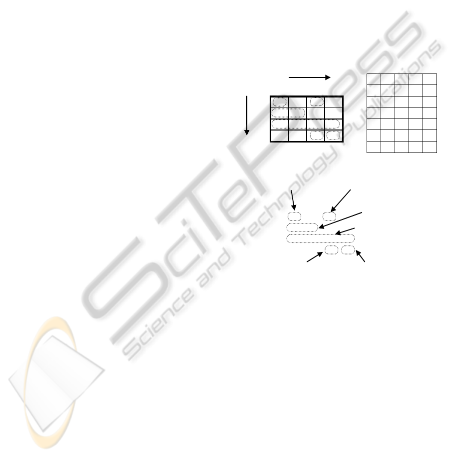
00 01 10 11
000 2
01 1 1
103333
11 4 0
ab
cd
!a!b!c!d !a!bc!d
!ab!c
abc!d
abcd
a!b
F
4
a b c d f
0 0 0 0 0 0
1 0 1 0 - 1
2 0 0 1 0 2
3 1 0 - - 3
4 1 1 1 0 4
5 1 1 1 1 0
a) b)
c)
Figure 1: (a) The map of integer function F
4
, (b) the
equivalent cube specification and (c) product terms.
Machine representation of single-output
Boolean functions frequently uses Binary Decision
Diagrams (BDDs), which can have many forms,
[Yanushkevich, 2006]. Integer-valued or multiple-
output Boolean functions are frequently represented
by Multi-Terminal Binary Decision Diagrams
(MTBDDs) or by BDD for the characteristic
function (BDD_for_CF), (Matsuura, 2007). The
latter type has a drawback of a large size because
input as well as output variables are used as decision
variables; it is also more difficult to work with.
From now on, we will therefore use only MTBDDs.
The DD size is the important parameter as it
directly influences the amount of memory storing
the DD data structure. However, the size of a DD is
MULTI-TERMINAL BDDS IN MICROPROCESSOR-BASED CONTROL
141

very sensitive to variable ordering and finding a
good order even for BDDs is an NP-complete
problem (Yanushkevich, 2006). The size of DDs for
random functions grows exponentially with the
number of variables n for any ordering, but functions
used in digital system design with few exceptions do
have a reasonable DD size. One exception is the
class of binary multipliers: for all possible variable
orderings, the BDD size is exponential for n-bit
inputs and 2n-bit output (Bryant, 1991).
We will refer to BDDs or MTBDDs with the
best variable ordering as to the optimal DDs. The
term a “sub-optimal DD” will denote a DD with a
size near to the optimal BDD.
3 MTBDD SYNTHESIS FROM
CUBE SPECIFICATION
In this section we present a heuristic technique for a
sub-optimal MTBDD synthesis. It is a generalization
of the BDD construction by means of iterative
disjunctive decomposition (Dvořák, 2007). Input
variables are selected one after another in such
a way that MTBDD cost is locally minimized.
Before formulation of the algorithm, we prefer
to illustrate the synthesis technique on the F
4
example in Fig. 2. The integer function z = F
4
(a, b,
c, d) of four binary variables is specified by cubes at
the top of Fig. 2. In the meantime we will select a
sequence of input variables for iterative decompo-
sition randomly, e.g. d, c, b, a. A single variable
(highlighted within tables in Fig. 2) will be removed
from the function in one decomposition step.
Starting with variable d, we inspect the set of input
cubes with value 0 or 1 in column d and look for all
possible compatible pairs of input cubes e = (e
1
, e
2
,
e
3
, 0) and e’ = (e’
1
, e’
2
, e’
3
, 1) hiding their values 0
and 1. One cube (...,0) may be compatible with
several cubes (...,1) and vice versa. These pairs will
be referred to as binary pairs (b-pairs).
Next we will identify input cubes with value "-"
in column d. From each such cube u = (u
1
, u
2
, u
3
, -)
we can create a compatible pair u = (u
1
, u
2
, u
3
, 0)
and u’ = (u
1
, u
2
, u
3
, 1) by substitution 0 and 1 for "-".
These pairs will be referred to as unary pairs (u-
pairs) because of their origin from one cube.
Remaining cubes of two types, q = (q
1
, q
2
, q
3
, 0) or
r = (r
1
, r
2
, r
3
, 1), are not compatible between them-
selves and neither with any cube in binary pairs; we
will call them orphaned input cubes. This is because
the compatible cubes q = (q
1
, q
2
, q
3
, 1) or r = (r
1
, r
2
,
r
3
, 0) map to the don´t care values and therefore are
not listed in the cube table. We can thus append each
orphaned cube with the identical invisible input cube
with DC output value. We will call these pairs
appended pairs (a-pairs).
In our example in Fig. 2 we will find
- only one b-pair, cubes 4&5
- two u-pairs, cubes 2&2 and 3&3
- two a-pairs, cubes 0&x, 1&x.
When we do decomposition of function F
4
by
removal of variable d,
F
4
= H(G(a, b, c), d), (3)
we have to intersect all b-, u-, and a-pairs of compa-
tible input cubes u = (u
1
, u
2
, u
3
) and v = (v
1
, v
2
, v
3
) in
order to obtain cubes of a residual function G and
map them into pairs of output values :
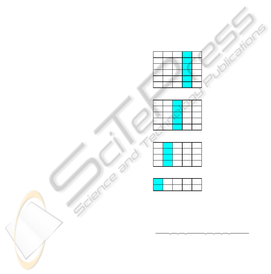
Figure 2: Iterative decomposition of an integer function F
4
of 4 binary variables (replacement of DC values in bold).
F
4
: u = (u
1
, u
2
, u
3
) F
4
(u
1
, u
2
, u
3
, 0) = P
F
4
: v = (v
1
, v
2
, v
3
) F
4
(v
1
, v
2
, v
3
, 1) = Q (4)
G: u* v = (z
1
, z
2
, z
3
) Z : = [P, Q]
For example, pair of values (4, 0) is produced by
cubes 4 and 5 in the first table in Fig.2; without
values of d are these cubes compatible and can be
replaced in the new table of a residual function G(a,
b, c) by a single input cube 111 – their intersection.
The removed variable d is left empty in all cubes of
the following tables. A pair of output values (4, 0)
from intersection of cubes 4&5 is replaced by a new
abcdz comp.
000000 cubes
100102 4&5 0:=(4,0)
2010- 1 2&2 1:=(1,1)
3 1 0 - - 3 3&3 2:= (3,3)
411104 0&x 3:=(0,
0
)
511110 1&x 4:=(2,
2
)
comp.
0111 0 cubes
1010 1 3&4 0:=(3,4)
210- 2 2&2 1:=(2,2)
3000 3 0&x 2:=(0,
0
)
4001 4 x&1 3:=(
1
,1)
comp.
000 0 cubes
1 1 0 1 0&3 0:= (0,3)
2 1 1 2 1&2 1:= (1,2)
301 3
comp.
00 0 cubes
1 1 1 0&1 0:= (0,1)
ICINCO 2010 - 7th International Conference on Informatics in Control, Automation and Robotics
142

integer id (0), as indicated in Fig. 2 by the
assignment 0 := (4, 0).
Unary pairs of cubes 2&2 and 3&3 produce
output pairs of the same values (1, 1) and (3, 3)
redefined to new identities 1 and 2. Finally input
cubes 0 and 1 are appended with the same invisible
cubes to produce output pairs (0, DC) and (2, DC).
Now the DC values must be defined so as not to
increase the number of already existing unique pairs.
If merging with one already found unique pair is not
possible, like in our case, we will use pairs of the
same values (0, 0) and (2, 2) and give them new
identities 3 and 4. Sometimes it may be useful to
replace all DC values by a special default value that
will be interpreted as "no _output" or "error".
Pairs of different output values correspond to a
true decision node, whereas pairs of the same output
values produce degenerate or false decision nodes,
because variable d in fact does not decide anything.
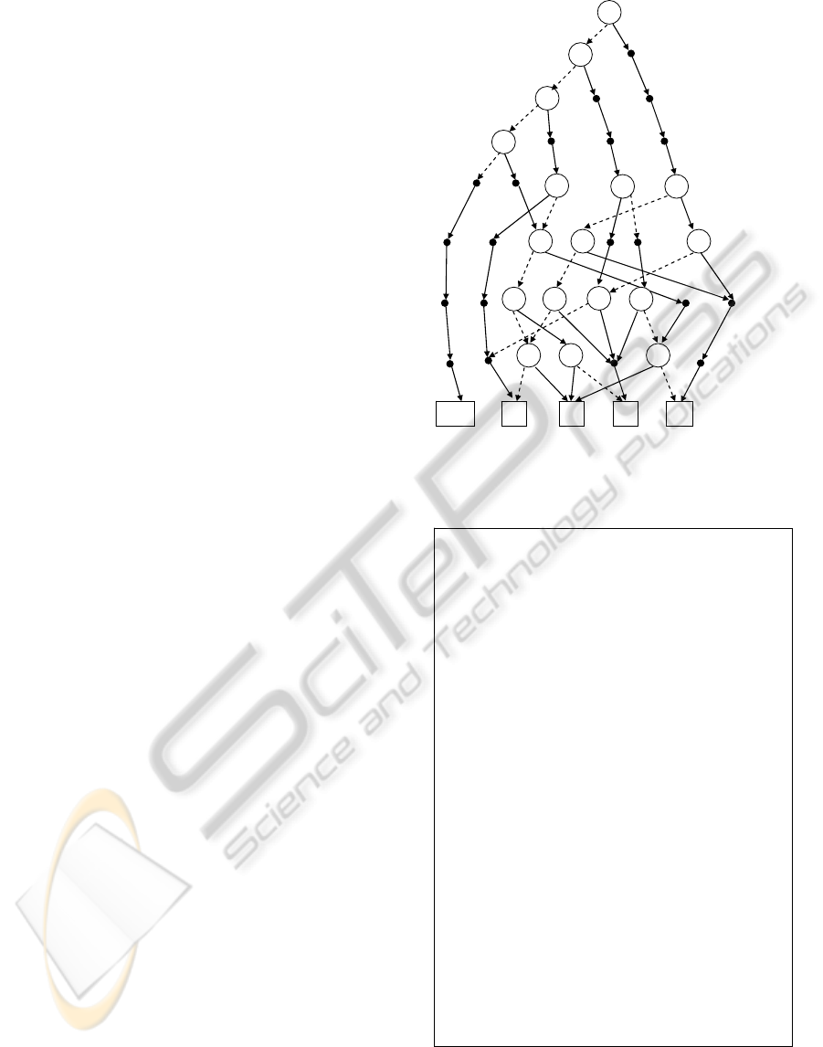
Nodes in the MTBDD are labeled by the new
identities of output pairs. There is one true node (0)
and four false nodes (1, 2, 3
and 4 shown as black
dots) in the lowest level of the MTBDD in Fig. 3.
Dashed edges are taken for 0-value and solid edges
for 1- or both values of decision variables.
0
0
0
3
2
0
2
1
3
4
3
1
2
0
a
b
c d
1
1
4
Figure 3: The MTBDD of function F
4
obtained by iterative
decomposition.
By now, we have exhausted all possible pairs of
compatible cubes of F
4
with d = 1 and d = 0 and
have replaced them by new shorter cubes of the
residual function G. The same procedure is repeated
in the following decomposition steps until all
variables have been removed. We move ahead in a
backward direction, from the leaves of the MTBDD
to its root, Fig. 3.
The remaining question not addressed as yet is,
which variable should be used in any given step. We
use a heuristic that strives to minimize the number of
true nodes t in the current level of the MTBDD. In
the case of a tie, a variable with a lower number of
false nodes f is selected. In case of a tie again, a
variable is chosen randomly.
The core of the above algorithm, the search for
the best variable in step i, i in 1 to n, is given below
(letters S stand for sets, M for tables):
// Determine the best variable v
k
in step k //
M
k-1
, a cube table of the (k1)
th
residual function;
(M
0
is the cube table of the original function);
S
v
, the set of input variables of the (k1)
th
residual
function;
v
k
, the best variable in step k;
v
best
← arbitrary variable from S
v
,
t
best
← size(M
k-1
), f
best
← 0;
for all variables v  S
v
do
M
p
← make b- and u-pairs(M
k-1
, v);
S
p
← unique_output pairs(M
p
);
S
m
← merge or add a-pairs(S
p
);
t ← #true nodes(S
m
);
f ←#false nodes(S
m
);
if (t < t
best
) or ((t == t
best
) and (f < f
best
))
then v
best
← v, t
best
← t, f
best
← f;
endif
endfor
v
k
← v
best
;
The whole algorithm for iterative decomposition has
been implemented in the SW tool HIDET (Heuristic
Iterative Decomposition Tool). It has been applied
successfully to a class of arbiter and allocator
circuits; parameters of some obtained MTBDDs are
given in Section 4.
4 BRANCHING PROGRAMS
WITH DISPATCH TABLES
Implementing multiple-output Boolean functions on
a microprocessor can be done in several ways.
Emulating PLC that evaluates one function after
another in a sum-of-products form by redundant
testing values of variables is slow and inefficient. A
better way makes use of the whole processor word
as 32 or 64 bits in parallel. The PLA matrix with n
inputs and m outputs can be emulated in n+m steps.
A product vector in the AND array is created by
accumulating contributions from input variables:
according to the value of an input variable, one of
two masks is logically multiplied with the product
vector created so far (and initially with all ones).
Then m outputs are generated serially applying a
single mask for each output to the product vector
MULTI-TERMINAL BDDS IN MICROPROCESSOR-BASED CONTROL
143

and detecting presence of at least a single 1.
However, if the number of cubes is larger than the
word size, above steps must be repeated several
times.
Finally, the method based on MTBDDs takes
always n or a fraction of n steps. Provided that a
(sub-)optimal MTBDD of a certain integer function
is known, writing a branching program is a routine.
We will illustrate it on the 4-input Round Robin
Arbiter (RRA) with 4 input request lines r
0
r
3
and 4
grant outputs g
0
g
3
. The n-bit priority register p
0
p
3
is maintained which points to the requester who is
next. It contains a single 1 that rotates one position
after a grant is issued. The MTBDD of this RRA
obtained by HIDET tool is in Fig. 4. The speed of
evaluation is given by the number of decision
variables tested simultaneously.
The sample of a symbolic program with testing
two binary inputs at a time is shown at Fig. 5. The
best performance is obtained by hand coding the
series of table lookups in assembly language and
replacing switch statements by dispatch tables. The
program uses 9 4-way and of 2 2-way dispatch
tables. The size of dispatch tables varies depending
on whether the input edge leads to a true decision
node (L1-L5, L7-L10) or passes through one or
more false nodes (L6, L11). In the assembly code,
the base address of a dispatch table gets modified in
two least significant bits by values of two variables
under the test. Items in a dispatch table contain
either the next base address or the terminal value.
One bit is used to differentiate between these two
formats. The total size of all dispatch tables is
94+22 = 40 words and an arbitration decision is
produced after four table lookups.
Had we used only single variable tests (a
branching program with 2-way tables), we would
need 17 dispatch tables of size 2, i.e. 34 words in
total. However, the performance would be 2- times
lower due to execution of a chain of 8 table lookups,
one in each level of the MTBDD. Faster processing
in three steps could test groups of 2, 3, 3 or 2, 2, 4
decision variables. The fastest execution would test
4 decision variables at a time and use 16-way
branching. The features of various options are
summarized in Table 1. The space  time product is
a figure of merit of quality of the implementation. It
gets the best (lowest) value for testing four variables
at a time.
With the aid of HIDET tool, MTBDDs of many
types of arbiters of different size have been obtained,
among others priority encoders, RR, LGLP (Last
Granted Lowest Priority) and LRS (Least Recently
Serviced) arbiters. Cube tables were obtained
automatically by means of small routines in C which
r3
r2
r1
r0
p1
p3
p2
p0
no_g g2 g1 g3
g4
0
0
1
0
2 1
0
1
2
0
1
4 3
0
3
4 1 2
0
3
1 2
4
0 2
1 3
L1
L2
L4
L3
3
2
5
4
5
6
7
6
5
6
L5
L8
L6
L10
L9
L11
L7
Figure 4: MTBDD of the 4-input RR arbiter
Figure 5: A symbolic program for the 4-input RRA.
enable scaling to the desired size. The results for
RRAn arbiters with n inputs, m outputs and specified
L1: inpu
t
x ←
r
3
r
2
; L10: inpu
t
x ←p
2
p
0
;
switch (x) { switch (x) {
case 0: case 0:
goto L2; output g
4
;
case 1: goto End;
goto L4; case 1:
case 2: output g
1
;
goto L5; goto End;
case 3: case 2:
goto L5; output g
3
;
} goto End;
L2: input x ←r
1
r
0
; case 3:
switch (x) { output g
3
;
case 0: goto End;
output no_g; }
goto End; L11: input x ←p
0
;
case 1: switch (x) {
goto L6; case 0:
case 2: output g
4
;
goto L3; goto End;
case 3: case 1:
goto L3; output g
1
;
} goto End;
… {
End:
ICINCO 2010 - 7th International Conference on Informatics in Control, Automation and Robotics
144

by #cubes are given in Tab. 2. The number of true
nodes multiplied by 2 gives the lower bound on
memory space (in words) for dispatch tables.
Table 1: Various RRA4 program options.
tested  dispatch # table space x
variables: table size lookups time
8 x 1 34 8 272
4 x 2 40 4 160
2, 3, 3 52 3 156
2, 2, 4 64 3 192
4, 4 72 2 144
8 256 1 256
Table 2: MTBDDs for Round Robin Arbiters.
in out
#cubes
bbb
# true
nodes
n m
RRA3 6 3 10 10
RRA4 8 4
17
17
RRA6 12 6
37
40
RRA8 16 8
65
75
RRA12 24 12
145
189
5 CONCLUSIONS
Programming a digital logic component of micro-
processor-based control systems need not rely only
on ladder diagrams anymore. Modern digital logic
design offers multi-terminal BDDs that can specify
groups of Boolean functions simultaneously, are
non-redundant and allow direct conversion to
branching programs with dispatch tables.
The advantages of the presented technique are
twofold:
1. The transition from cube specification to the
MTBDD and then to the assembly program is
relatively easy and can be automated. The latter
transition is of course depending on a target
processor.
2. As soon as the MTBDD is known, the most
suitable program implementation can be chosen
trading-off performance for memory space (mainly
to store dispatch tables).
The programming technique has been demonstrated
on (but it is not limited to) the class of arbiter
circuits. Currently it is applicable to integer
functions of Boolean variables with don´t cares.
Future research will address multiple-output
Boolean functions with compatible input cubes and
incidentally with ternary output cubes c  {0, -, 1}
m
.
This extension could provide appropriate design
techniques for new classes of functions.
ACKNOWLEDGEMENTS
This research has been carried out under the
financial support of the research grants “Natural
Computing on Unconventional Platforms”,
GP103/10/1517, “Safety and security of networked
embedded system applications”, GA102/08/1429,
"Mathematical and Engineering Approaches to
Developing Reliable and Secure Concurrent and
Distributed Computer Systems" GA 102/09/H042,
all care of Grant Agency of Czech Republic, and by
the BUT FIT grant FIT-10-S-1 and the
research plan MSM0021630528.
REFERENCES
Bryant, R. E., 1991. On the complexity of VLSI
implementations and graph representations of Boolean
functions with applications to integer multiplication. In:
IEEE Transactions on Computers, Vol. 40, pp. 205–213,
1991.
Brzozowski, J. A., Luba, T., 1997. Decomposition of
Boolean Functions Specified by Cubes. Research report
CS-97-01, University of Waterloo, Canada, p. 36.
Dvořák, V., 1997. Efficient Evaluation of Multiple-
Output Boolean Functions in Embedded Software or
Firmware, In: Journal of Software, Vol. 2, No. 5, 2007,
pp. 52–63.
Gilvarry, I., 2009.
IA-32 Features and Flexibility for
Next-Generation Industrial Control. Intel Technology,
Journal, Vol. 13, Issue 01, March 2009.
Matsuura, M., Sasao, T., 2007. BDD representation
for incompletely specified multiple-output logic functions
and its application to the design of LUT cascades, In:
IEICE Transaction on Fundamentals of Electronics,
Communications and Computer Sciences, Vol. E90-A,
No. 12, Dec. 2007, pp. 2770–2777.
Petruzella, F.D., 2004. Programmable Logic Control-
lers, McGraw Hill Science/Engineering/Math,
Sosic, R., Gu, J. and Johnson, R., 1996. The Unison
algorithm: Fast evaluation of Boolean expressions. ACM
Transactions on Design Automation of Electronic Systems,
1(4): pp. 456-477, Oct. 1996.
Yanushkevich, S. N., Miller, D. M., Shmerko, V.P.,
Stankovic, R. S., 2006. Decision Diagram Techniques for
Micro- and Nanoelectric Design Handbook. CRC Press,
Taylor & Francis Group, Boca Raton, FL.
MULTI-TERMINAL BDDS IN MICROPROCESSOR-BASED CONTROL
145