A HYBRIDIZED GENETIC ALGORITHM FOR COST

ESTIMATION IN BRIDGE MAINTENANCE SYSTEMS

Khaled Bashir Shaban

Department of Computer Science and Engineering, College of Engineering, Qatar University, Doha, Qatar

Abdunnaser Younes, Nathan Good, Mohammed Iqbal and Richard Lourenco

Department of Systems Design Engineering, Faculty of Engineering, University of Waterloo, Canada

Keywords: Hybridized Genetic Algorithm, Cost Estimation, Bridge Maintenance Systems.

Abstract: A hybridized genetic algorithm is proposed to determine a repair schedule for a network of bridges. The

schedule aims for the lowest overall cost while maintaining each bridge at satisfactory quality conditions.

Appreciation, deterioration, and cost models are employed to model real-life behaviour. To reduce the

computational time, pre-processing algorithms are used to determine an initial genome that is closer to the

optimal solution rather than a randomly generated genome. A post-processing algorithm that locates a local

optimal solution from the output of the genetic algorithm is employed for further reduction of computational

costs. Experimental work was carried out to demonstrate the effectiveness of the proposed approach in

determining the bridge repair schedule. The addition of a pre-processing algorithm improves the results if

the simulation period is constrained. If the simulation is run sufficiently long all pre-processing algorithms

converge to the same optimal solution. If a pre-processing algorithm is not implemented, however, the

simulation period increases significantly. The cost and deterioration tests also indicate that certain pre-

processing algorithms are better suited for larger bridge networks. The local search performed on the

genetic algorithm output is always seen as a positive add-on to further improve results.

1 INTRODUCTION

There is an increasing need for immediate and long-

term infrastructure renewal of provincial and

municipal highways and roads, buildings, water

supply systems, wastewater treatment facilities,

sanitary and storm sewers, and bridges and

overpasses. The gross value of these assets

amounted to $286.2 billion in 2007. The need of the

renewal is caused in part by the large scale boom in

infrastructure that occurred 30 to 60 years ago. The

average life of these structure ranges from 28.2 years

for highways and roads to 43.3 years for bridges and

overpasses (CBC News, 2008). As such,

governments have the arduous task of budgeting for

a backlog of repairs and reconstructing of existing

infrastructure. To limit the current budgets,

alternative systems are presented to seek the optimal

cost per cycle solutions to support the repair or

reconstruction of the aging infrastructure.

Once built, bridges receive little maintenance,

unlike other infrastructures, such as roads and water

infrastructure, which are maintained or repaired

periodically. Changing weather conditions and the

steady rise in traffic levels have caused existing

bridges to depreciate at a much higher rate.

According to a 2006 Statistics Canada study, bridges

are at 49% of their useful life (Charles Mandel,

2007). Saeed Mirza in (Charles Mandel, 2007) states

that the current situation is disastrous and estimates

that $100 billion should be invested to upgrade

existing bridges and other infrastructure. A 2007

report issued by the Residential and Civil

Construction Alliance of Ontario warns that 40% of

Ontario’s bridges will require significant repair over

the next few years (Bruce Campion-Smith, 2007).

The catastrophic collapse of the I-35 Bridge in

Minneapolis, Minnesota on August 2, 2007 has

increased public awareness of the importance of

maintaining bridges. Clearly there is an increasing

need to invest in bridge infrastructure.

428

Shaban K., Younes A., Good N., Iqbal M. and Lourenco R. (2010).

A HYBRIDIZED GENETIC ALGORITHM FOR COST ESTIMATION IN BRIDGE MAINTENANCE SYSTEMS.

In Proceedings of the 12th International Conference on Enterprise Information Systems - Artiﬁcial Intelligence and Decision Support Systems, pages

428-433

DOI: 10.5220/0002974304280433

 SciTePress

Traditionally, in bridge maintenance systems

(BMSs), experts use their judgment and experience

to determine which bridges to repair and the extent

of repair each year. However, as the number of

bridges increases, this task evolved into a complex

optimization problem that is well beyond the

abilities of even the most experienced experts. In

fact, this problem is a nondeterministic polynomial

(NP) problem, which is computationally intractable

for traditional methods. Genetic Algorithms (GAs)

have been shown to be effective in solving NP-hard

problems, and thus are good candidates for solving

this problem.

The bridge inventory contains a list of all the

bridges in the network. Each bridge component has a

condition rating. The deterioration and improvement

models quantify how much the bridge components

degrades or improves its condition each year,

depending upon whether a repair takes place or not.

The cost model determines how much a repair will

cost. This model depends on the current condition

rating of the bridge. All models occur over a

predetermined time period. The evolutionary

algorithms try to optimize (minimize) the total cost

spent over the time period. The total cost is

optimized by determining which bridges to repair

and which components on the bridge to repair.

2 A HYBRIDIZED GA FOR COST

ESTIMATION IN A BMS

The GA derives a solution based on a fitness

function and constraints. Parameters such as

mutation rate, the number of generations and

crossover rate are also to be tuned. The fitness

function is to minimize the overall repair cost for the

bridge network over the desired time period. The

overall repair cost is calculated by summing the

costs for each year. The other option was to make

the fitness function based on the quality of the

bridges. However, due to safety considerations, the

bridge quality was deemed better suited as a hard

constraint. Several constraints were added to the

implemented system including:

1. Repairs Constraint:

A bridge can only be repaired maximum of two

times over a 5 year period, or 5 times over a 20 year

period. This constraint reflects real life constraints.

Bridges that are repaired constantly incur higher

costs (both construction costs and user costs).

2. Condition Constraint:

The condition of a bridge cannot fall below 30. Fur-

thermore, a bridge cannot be repaired if its condition

exceeds 90. These conditions maintain a satisfactory

bridge quality level and eliminate the possibility of

repairing well-conditioned bridges.

3. Cost Constraint:

A predefined yearly budget is be defined. The yearly

budget is related to the number of bridges within the

system. This constraint reflects real life budget

restraints.

In order to reduce the time to develop an

acceptable solution, some pre-processing of the data

must take place. The initial data set that the GA uses

to optimize the fitness function should be

conditioned to be within the ball park of the final

solution. For example, we know that in any given

year, because of budgetary limits, only several

bridges are repaired. Therefore, the GA chromosome

(i.e. bridges to repair) will initially be setup to repair

only a small percentage of the bridges per year. In

order to determine these initial values, we will use

fuzzy sets, among other approaches (to be

investigated). The fuzzy set outputs will be no

repair, light repair, medium repair and extensive

repair. They will correspond to the condition of the

bridge – the input fuzzy sets.

A post-processing algorithm can be used to

locate a local optimal solution. Genetic algorithms

are capable of determining the optimal solution.

However, even with the inclusion of pre-processing,

determining the optimal solution may take a

substantial amount of time. The post-processing

algorithm can determine a better solution by slightly

altering the bridge repair schedule (represented as

the genome). For example, if a heavy repair is made

in year X for a bridge, the post-processing algorithm

can determine if a local optimal solution is found by

downgrading the repair severity to a medium or light

repair, or altering the time or repair to year X+1 or

year X−1. The post-processing algorithm can also be

used to check the output from the genetic algorithm.

An emphasis is made to limit the computations

required for the post-processing algorithm.

2.1 Pre-processing

The motivation behind pre-processing the genome is

to reduce the computational time required to produce

the optimal solution. Four pre-processing algorithms

were implemented.

The first algorithm randomly generates genome.

For any bridge/year combination, it has a 5% chance

of assigning a level 1 repair, a 3% chance of

assigning a level two repair, a 2% chance of

assigning a level three repair, and a 90% chance of

A HYBRIDIZED GENETIC ALGORITHM FOR COST ESTIMATION IN BRIDGE MAINTENANCE SYSTEMS

429

assigning no repair at all.

The second algorithm repairs 10% of the bridges

every year. If the bridge’s quality is below 35 it

assigns a level 3 repair. If the quality is between 35

and 50, it assigns a level 2 repair. If the quality is

above 50, it assigns a level 1 repair. After assigning

the repairs for each year, it recalculates the bridge

qualities for the subsequent years.

The third algorithm will repair any number of

bridges. If the bridge’s quality falls below 40, it will

be repaired. Given a five year study if this occurs in

the first year, a level 3 repair will be assigned. If the

quality falls below 40 in the second or third year, a

level 2 repair will be assigned. If it falls below 40 in

the fourth or fifth year, a level 1 repair will be

assigned.

The fourth algorithm repairs a set number of

bridges each year. Given a five year study, three

bridges are repaired each year. It applies a level 2

repair to the worst bridge and level 1 repairs to the

other two bridges. It will not repair a bridge unless it

is below a quality of 50 and will not repair the same

bridge twice.

2.2 Post-processing

It was noticed during the testing that even with a

relatively small study size, the genetic algorithm

took a very long time to converge to the optimal

solution (6-7 hours). In order to combat this, a post-

processing algorithm was implemented. In these

cases, the post-processing algorithm can be run on

any results the GA produced before it was stopped to

improve upon those results.

The post-processing algorithm looks at each

repair that is being made, and examines the effect of

lowering it one level (e.g. level 3 repair to level 2, or

level 1 to no repair). If lowering the repair level does

not cause any bridge to fall below the quality

threshold of 30, it will be lowered. Otherwise it will

be kept at the same level. This is a local search that

is used to refine the genetic algorithm results.

2.3 Appreciation Model

After a repair, the quality of the bridge will increase.

The amount of increase is dependent on the severity

of the repair. There are three levels of repair in the

proposed system: light repair, medium repair, and

heavy repair. Light repair is used to recondition the

bridge elements; this includes but is not limited to

resurfacing the deck. Medium repair is used to

replace elements within the bridge. Elements can

include joints within the bridge structure. Heavy

repair is used to replace most of the bridge.

Given the limited information on the

deterioration of the bridges, all three types of repair

will produce a static improvement in the bridge

quality. For example, if a light repair is used on

bridge A, the quality of bridge A will increase by ten

points. A medium repair will result in an increase of

30 points. Heavy repair results in an increase of 50

points. All three types of repair are independent of

the age and existing condition of the bridge. The

maximum bridge quality after any repair is 90.

The formula used to calculate the condition of a

bridge after a repair is made is shown below and

Table 1 lists the i

and I constants for each repair

level.

where:

C bridge condition

P previous bridge condition

i condition improvement percentage

I bridge improvement

CP( i I





(1)

Table 1: Appreciation Model Constants.

Repair Level i

Light 15% 10

Medium 20% 30

Heavy 30% 50

2.4 Deterioration Model

The deterioration of the bridge is the process of

decline from its original condition under normal

operating circumstances (Abed-Al-Rahim, I. and

Johnston, W., 1995). This process excludes rare

phenomena such as natural disasters and includes

physical and chemical changes (Hatem Elbehairy,

2007) (Yang, Ming-Wing, 2007). Examples of each

include general wear to components of the bridge

like the deck and the bridge’s joints, and rusting on

bridge members.

Common factors which affect the rate at which a

bridge will deteriorate include the bridge’s age, the

average traffic levels, exposed environment

conditions, the design of the bridge, and the quality

of the material used to construct the bridge. The only

available information for this study is the bridge’s

age, its current depreciation, and it’s expected

remaining lifespan. As such, the depreciation model

will only reflect these parameters.

For this study a mechanistic deterioration model

(Hatem Elbehairy, 2007) will be employed. A

mechanistic model employs a known nonlinear

relationship in the form of Equation 2. The

mechanistic deterioration model is simple to

ICEIS 2010 - 12th International Conference on Enterprise Information Systems

430

implement and computationally inexpensive. The

values of A and B can be assigned or determined

using fuzzy inference. The mechanistic model

reflects changing deterioration per year, where the

deterioration rate decreases as the bridge gets older.

()

Ct Ae





(2)

Since the deterioration of the bridge is the

process of decline from its original condition under

normal operating circumstances, a simple decaying

exponential was used to approximate the

deterioration. In the formula used to calculate

deterioration shown in equation (2), the deterioration

is related to deterioration rate provided in the

original data. The inclusion of the deterioration rate

reflects the different rate of decay for each bridge.

The multiplier is a constant for each bridge. The

multiplier was modified until it conformed to a

deterioration rate found in various literature sources

on the subject.

The deterioration and appreciation models were

combined to produce a single model which updates

the condition of the bridges on a yearly basis.

where:

C bridge condition

P previous bridge condition

d deterioration rate

m multiplier

CPe





(3)

2.5 Cost Model

The cost model is used to determine the costs

associated with repairing a bridge within the

network of bridges. Generally there are two cost

models associated with a BMS: the user cost model

and the repair cost model. The cost model used in

our approach will only look at repair costs. User

costs are extra costs which are paid by the bridge

user (i.e. financial cost of time spent in traffic). User

costs are omitted from our approach because they

are generally subjective.

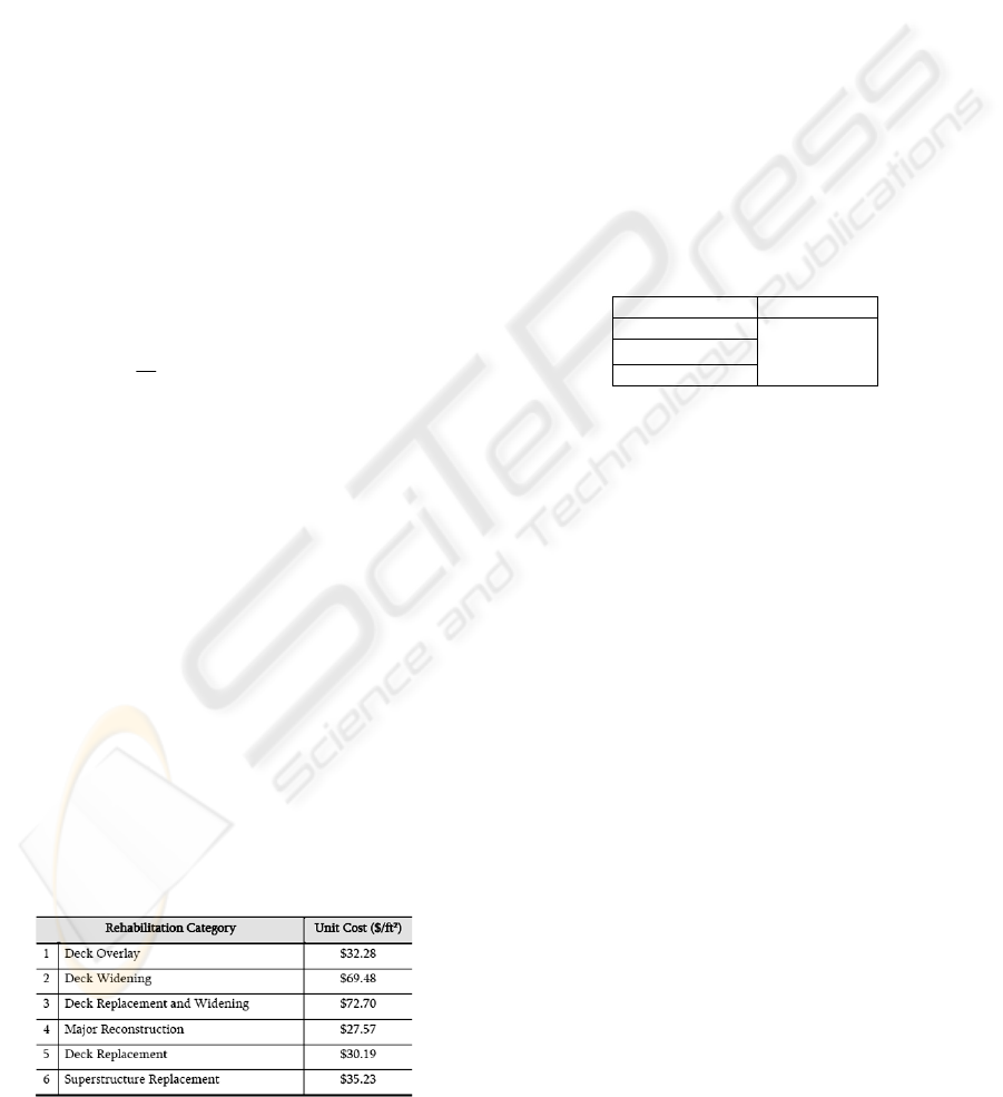
Table 2: Repair Unit Costs.

The repair costs can be expressed either as a unit

cost or a percentage of the initial cost of the bridge.

Unit costs are associated with the costs of repairing

individual items of the bridge (Saito, M., and Sinha,

K., 1990). An example of user costs is shown in

Table 2. Our approach will determine the cost of

repair as a percentage of the initial cost. This

approach is less computational. Furthermore the

limited information provided for each bridge makes

the unit cost approach impossible to implement.

The formula to calculate the cost of a repair is

based on the initial construction cost of the bridge,

which was provided. The formula for the repair cost

is shown below and Table 3 lists the multiplier

constants for each repair level.

where:

RC repair cost

C construction cost (specified for each bridge)

M repair type multiplier

RC CM



(4)

Table 3: Cost Model Constants.

Repair Level M

Light 0.1

Medium 0.4

Heavy 0.6

3 EVALUATION

Testing is focused on finding the best pre-processing

algorithm. The first step was to establish a set of

testing conditions which would allow us to properly

compare the different algorithms. We then changed

the testing conditions to observe the effect on the

optimal solutions.

To keep our testing consistent, we needed to fix

the number of bridges (study sample size) and the

number of years (study period). Although we had

data for 161 bridges, and could extrapolate the

bridge quality for any number of years using the

deterioration and appreciation models, we elected to

use a sample of 20 bridges over a 5 year period. The

crossover and mutation rate used for the genetic

algorithm was set at 0.5 and 0.1 respectively.

As mentioned, the main testing parameter will be

the pre-processing type. In addition to testing the

effectiveness of each pre-processing type, additional

tests will be conducted to determine the effects of

changing the deterioration rate and costs.

3.1 Pre-processing Algorithms

Comparison

Although we created four pre-processing algorithms,

A HYBRIDIZED GENETIC ALGORITHM FOR COST ESTIMATION IN BRIDGE MAINTENANCE SYSTEMS

431

the first one, which was random, either failed to find

valid solutions or took a very long time to do so in

our testing. As a result, we concluded that this was

not a suitable method for pre-processing (as

expected) and focussed our attention on the

remaining three algorithms.

In order to compare the effectiveness of the three

remaining pre-processing algorithms, tests were run

that involved setting all the variables in the system

constant while only changing the pre-processing the

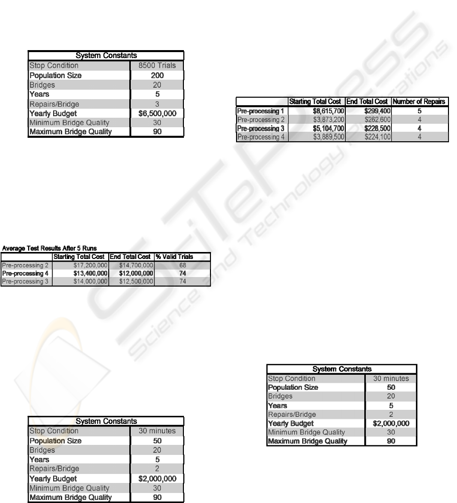
algorithm. Table 4 shows the systems settings for the

initial comparison.

Table 4: Initial Pre-Processing Comparison Settings.

Looking at the above table we see that the tests

were run for 8500 trials, which is a relatively short

period of time but sufficient enough to show a

system trend. Table 5 shows the results obtained

from running the tests with each pre-processing

algorithm over 5 runs.

Table 5: Initial Pre-Processing Results.

We can see that pre-processing algorithm 2 starts

in a state with the lowest total cost, among the three,

and finishes with the lowest total cost. Similarly, the

first pre-processing algorithm has the highest staring

and end total cost. This indicates that, with all

variables set, the quality of the starting state dictates

how good the end state will be, in a given amount of

time.

Table 6: Optimized Pre-Processing Constants.

Of course, over a long enough time period all

solutions will converge to a global optimum, but our

concern is to determine which method will do this

the quickest or which method will produce the best

result in a given time frame.

To confirm that all methods will converge to an

optimum the tests were run for much longer. The

new systems constants are shown in Table 6.

The stop condition was changed from 8500 trials

to 30 minutes. The population size was reduced to

50 to reduce the consumption of computer memory.

The bridge repairs per year and yearly budget

constraints were reduced to find a solution with

fewer repairs. The random pre-processing algorithm

was also included. The test results are summarized

in Table 7.

Table 7: Optimized Pre-Processing Results.

The total cost converges to around $200,000 for

all of the pre-processing algorithms. This clearly

shows that there is a global optimum that is

eventually reached.

3.2 Other Parameter Testing

Changes to the cost and the deterioration models

were made to evaluate the effects on the optimal

solution determined in section 2.2. The random pre-

processing method was omitted from both tests.

The first test was to determine the effect of

changing the cost model. The repair type multiplier

for light repairs was changed to 0.2. Table 8 displays

the system constants used for the test. The test

results are shown in Table 9.

Table 8: Test Constants for Cost Model Testing.

The second test was to determine the effect of

changing the deterioration model. The deterioration

multiplier was changed from 10 to 5. Table 10

displays the system constants used for the test. The

test results are shown in Table 11.

ICEIS 2010 - 12th International Conference on Enterprise Information Systems

432

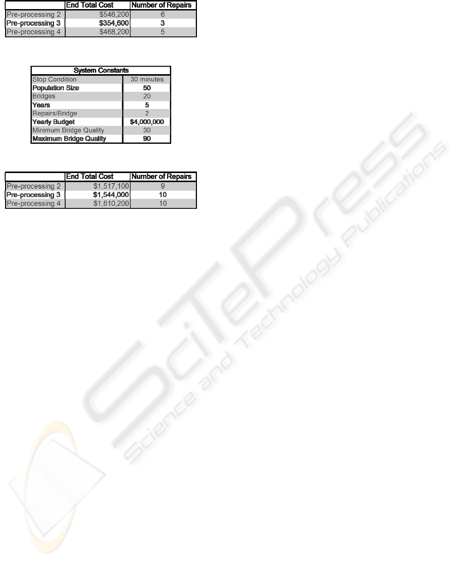
Table 9: Test Results for Cost Model Test.

Table 10: Test Constants for Deterioration Model Testing.

Table 11: Test Results for Deterioration Model Test.

As expected, the optimized total costs increased

for both tests. A more profound discovery is that the

pre-processing 2 algorithm outperformed the other

two algorithms for the deterioration model test. By

increasing the multiplier, the deterioration per year

increased significantly. As a result more bridges

required repair. Pre-processing algorithm 2 is better

equipped at handling larger bridge repair demands

since it is capable of repairing a constant number of

bridges per year. Pre-processing algorithms 3 and 4

will only repair the lowest quality bridges. If there is

a large number of bridges that fit this criterion in a

single year the algorithm may have difficulties

addressing all the bridges.

3.3 Post Processing Results

To demonstrate the effectiveness of the post-

processing algorithm, it was applied to the three

simulations for the network of 20 bridges over a five

year study term. The cost improved from $224,000

to $7,800.

4 CONCLUSIONS

Experimental tests showed that when a pre-

processing algorithm was applied prior to the genetic

algorithm, the genetic algorithm was able to obtain a

better solution in a fixed period of time than when

no pre-processing took place. More specifically, pre-

processing algorithms 3 and 4 generally resulted in

the best performance. However, when the

deterioration model was modified to increase the

rate of bridge deterioration, pre-processing

algorithm 2 was the top performer. This shows that

pre-processing algorithm two is the most flexible of

those tested. This is important, as different

municipalities or government may have very

different models for appreciation, depreciation and

repair cost. Pre-processing algorithm 2 is best

equipped to deal with these variations as the number

of bridges repaired is not static (as is the case in pre-

processing algorithms 3 and 4).

A post-processing algorithm was devised to

improve upon the genetic algorithm solution. While

the algorithm was implemented and preliminary

tests showed that it was successful in improving

upon the solution obtained by the genetic algorithm,

more testing is required with a wider range of

conditions to confirm that the post-processing

algorithm is effective.

REFERENCES

CBC News, 2008, Feb 13, “Average age of highways and

roads down, age of bridges up: Stats Can,” [Online

Article], [cited 2008 March 14], Available at:

http://www.cbc.ca/canada/story/2008/02/13/public-

infrastructure.html

Charles Mandel, 2007, Aug 2, CanWest News Service,

“Canada could face infrastructure crisis: expert,”

[Online Newspaper Article], [cited 2008 March 14],

Available at: http://www.canada.com/montrealgazette/

news/story.html?id=33cf9d88-98b0-41d7-b125-6b43

ed98fff9

Bruce Campion-Smith, 2007, Nov 20, The Star,

“Infrastructure 'near collapse',” [Online Newspaper

Article], [cited 2008 March 14], Available at: http://

www.thestar.com/News/Canada/article/278129

Hatem Elbehairy, 2007, “Bridge Management Systems

with Integrated Life Cycle Cost Optimization.” PhD

Thesis, University of Waterloo, Ontario, Canada, pp.

15-40.

Abed-Al-Rahim, I. and Johnston, W., 1995, “Bridge

Element Deterioration Rates”, Transportation

Research Record, 1490, Transportation Research

Board, pp.9-18.

Bolukbasi, M., Arditi, D., and Mohammadi, J., 2006,

“Deterioration of Reconstructed Bridge Decks“,

Structure and Infrastructure Engineering, 2 (2), pp.

23-31.

Saito, M., and Sinha, K., 1990, “Data Collection and

Analysis of Bridge Rehabilitation and Maintenance

Costs”, Transportation Research Record, 1276, pp.72-

75.

Yang, Ming-Wing, 2007, “A Comparison of Neural

Network, Evidential Reasoning, and Multiple

Regression Analysis” in Modelling Bridge Risks.

pp.336-348.

A HYBRIDIZED GENETIC ALGORITHM FOR COST ESTIMATION IN BRIDGE MAINTENANCE SYSTEMS

433