
EMD OVERSHOOT EFECT IN ERP DETECTION
ERP Detection related Specifics of the Empirical Mode Decomposition in EEG
Analysis
Jindrich Ciniburk
Department of Computer Science and Engineering, University of West Bohemia, Univerzitni, Pilsen, Czech Republic
Keywords:
Hilbert Huang transform, HHT, Empirical mode decomposition, EMD, Event related potentials, ERP, Signal
processing, Electroencephalography, EEG.
Abstract:
Event related potentials (ERPs) are detected from continuous EEG. Most common method for ERPs detection
is averaging. But this method is not suitable for single trial detection, because it requires lot of epochs. When
we are performing attention experiments, it is required to detect ERPs ideally from single epoch. To detect
ERP means determine its amplitude and latency. EEG signal is quasi-stationary therefore it is necessary to use
signal processing methods designed for this task. We decided to use Hilbert-Huang transform. Its capabilities
and problematic for ERP detection are discussed in the paper.
1 INTRODUCTION
Event Related Potentials (ERPs) play the main role in
the Brain-Computer Interface, in the medicine and at-
tention experiments. Our laboratory is focused on as-
sessment of drivers attention. We cooperate with the
University Hospital in Pilsen, Skoda Auto Inc., and
Faculty of Transportation Science of Czech Technical
University in Prague.
Our experiments are performed in the commercial
simulation software Virtual Battlespace. Continuous
EEG with stimuli marks is recorded during experi-
ments. The marks provide information when each
stimulus comes and where is ERP wave in the EEG
signal. The short time period after stimulus is called
epoch. The interval between stimulus and ERP wave
is called latency, see (Luck, 2005; Sanei and Cham-
bers, 2007).
For correct evaluation of our experiments results,
it’s fundamentalto precisely determine amplitude and
latency of ERP waves.
2 HILBERT-HUANG
TRANSFORM
Hilbert-Huang transformation was designed to ana-
lyze data which are nonlinear and nonstationary. This
method was proposed by Huang in (Huang and et al.,
Figure 1: ERP wave is described by its latency and ampli-
tude.
1998). It consists of empirical mode decomposition
(EMD) and the Hilbert spectral analysis (HAS) meth-
ods, both of these methods were introduce by Huang
et al.
2.1 Intrinsic Mode Functions
An intrinsic function (IMF) is function which has to
fulfill following two conditions:
1. In the whole data set, the number of extremes and
the number of zero crossings must be either equal
or differ by one at most.
2. The mean value of the envelope defined by the
local maxima and the local minima is zero at any
point (Liu, 2002; Huang and et al., 1998).
An IMF represents simple oscillatory mode as coun-
terpart to a simple harmonic function, but it is much
more general by its definition. The conditions which
238
Ciniburk J. (2010).
EMD OVERSHOOT EFECT IN ERP DETECTION ERP - Detection related Specifics of the Empirical Mode Decomposition in EEG Analysis.
In Proceedings of the 12th International Conference on Enterprise Information Systems - Human-Computer Interaction, pages 238-241
DOI: 10.5220/0002975302380241
Copyright
c
SciTePress

IMF fulfills are necessary for defining instantaneous
frequency.
2.2 Empirical Mode Decomposition
The goal of the empirical mode decomposition is to
decompose original data (signal) to the IMFs and the
residue. The most of the data are not IMFs. At any
time, the data may involve more than one oscillatory
mode. That is why simple Hilbert transform cannot
provide the full description of the frequency. The pro-
cess of acquiring the IMFs is called sifting and it’s de-
scribed below (Qu and Wu, 2008; Huang and Attoh-
Okine, 2005):
1. Initialize the residue to the original signal r
0
(t) =
x(t) and IMF counter i = 1
2. Extract the i-th IMF:
3. Initialize h
0
(t) = r
i−1
(t) and initialize step
counter k = 1
4. Locate local maxima and minima in h
k−1
(t)
5. Create upper envelope by connecting detected
maxima with cubic spline
6. Create lower envelope by connecting detected
minima with cubic spline
7. Calculate the mean m
k−1
(t) by averaging the up-
per and lower envelopes
8. Calculate h
k
(t) = h
k−1
(t) − m
k−1
(t)
9. Check stopping criteria
10. If stopping criteria are satisfied then IMF
i
(t) =
h
k
(t)
11. Else k = k+ 1 and continue with 4
12. New residue is r
i
(t) = r
i−1
(t) − IMF
i
(t)
13. Check stopping criteria of EMD
14. If r
i
(t) has at least 2 extremes then i = i + 1 and
continue with 2
15. Else the decomposition is finished and r
i
(t) is the
residue after decomposition
2.3 EMD Stopping Criteria
During EMD we want to retrieve IMFs described in
chapter 2.1. These functions have to fulfill two con-
ditions. The second condition (mean of the envelopes
is meant to be zero) is very difficult to fulfill. As the
points 4 to 9 of the EMD (from chapter 2.2) are re-
peated, the mean approaches to zero. But this makes
amplitude variations of the individual waves more
even. When we want to achieve strictly zero mean,
we can assume that the amplitudes become constant
and we lose very important information of the signal.
So there were proposed two stoppage criterions. One
original proposed in (Huang and et al., 1998) equation
1.
SD =
T
∑
t=0
|h
k−1
(t) − h
k
(t)|
2
h
2
k−1
(t)
(1)
Alternative for the first one is similar to Cauchy con-
vergence test:
SD =
∑
T
t=0
|h
k−1
(t) − h
k
(t)|
2
∑
T
t=0
h
2
k−1
(t)
(2)
The sifting process will stop, when the SD is smaller
than the selected threshold. The second stoppage cri-
terion is based on the S-number which is defined as
the number of consecutive sifting when the number
of zero-crossings and extremes are equal or differs by
one at most.
2.4 The Hilbert Spectrum
Hilbert transform (Mathworks, 2010; Marple, 1999)
returns the analytic signal from real data sequence.
The analytic signal x = x
r
+ i · x
i
has its real part,
x
r
which represents the original data, and its imag-
inary partx
i
, which contains the Hilbert transform.
The imaginary part is a version of the original real
sequence with a 90 phase shift. Sines are therefore
transformed to cosines and vice versa. The Hilbert
transformed series has the same amplitude and fre-
quency content as the original real data and includes
phase information that depends on the phase of the
original data. The Hilbert transform is useful for cal-
culating instantaneous attributes of time series, espe-
cially the amplitude and frequency. The instantaneous
amplitude is the amplitude of the complex Hilbert
transform; the instantaneous frequency expresses the
rate of change of the instantaneous phase angle. In
case of a pure sinusoid, the instantaneous amplitude
and frequency are constant.
3 EMPIRICAL MODE
DECOMPOSITION OF EEG
When the EMD is performed on the data series, we
are trying to create upper and lower envelopes by con-
necting local extremes with cubic spline. Though,
some difficulties surface in the process. When we
want to create an envelope which covers whole signal,
we have to realize that the first (last) extreme point is
not present in the data at all. So, the closest extreme
to the beginning or the end of the signal belongs to
the upper or lower envelope. Then the second closest
EMD OVERSHOOT EFECT IN ERP DETECTION ERP - Detection related Specifics of the Empirical Mode
Decomposition in EEG Analysis
239
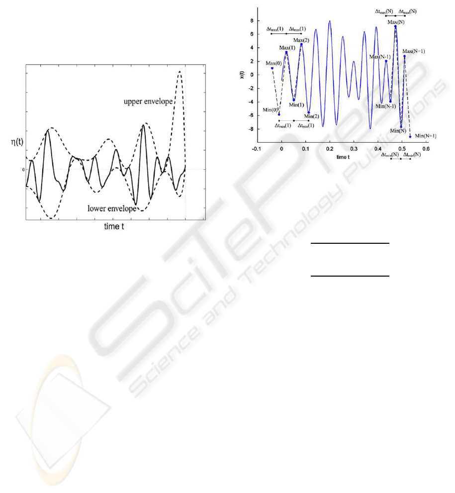
extreme is the point from where the both envelopes
are defined.
So we have to add additional extreme points to ex-
tend the envelopes over the whole signal. But it is the
tricky part. We have to position them very carefully,
because their incorrect location leads to imprecise es-
timate of the cubic spline (2.). This overshoots or un-
dershoots don’t describe characteristics of the signal,
but they could be propagated inward and corrupt the
whole signal. The problem is described in detail in
(D˝atig and Schlurmann, 2004). To restrain this effect,
Figure 2: Example of overshoot from (D˝atig and Schlur-
mann, 2004).
several methods of additional extreme selection were
proposed. They are described in following chapters.
3.1 Mirror Method
Mirror method was proposed by Rilling and described
in (Qu and Wu, 2008). The procedure is very simple.
Additional extremes are mirror symmetric to the ex-
tremes that are closest to the beginning or end of the
signal. The algorithm follows:
1. Locate the extreme closest to the begin of the sig-
nal (we found Max(1) ). Then locate the extreme
closest to Max(1), this is Min(1)
2. Create new extreme on the begin of the data
by creating Min(0) respecting the mirror symme-
try. Min
x
(0) = Max
x
(1) − (Min
x
(1) − Max
x
(1)),
Min
y
(0) = Min
y
(1)
3.2 Slope based Method
Slope based method was proposed in (D˝atig and
Schlurmann, 2004) and described in (Qu and Wu,
2008). This method also extends extremes, but add
one minimum and one maximum to the beginning
or end of the signal. The new extremes are gener-
ated using two mathematically defined slopes created
through the extremes. These slopes are derived from
the distances between successive minima and maxima
and from amplitude differences. In the first step we
Figure 3: The illustration of the slope based method from
(Qu and Wu, 2008).
have to calculate the slopes s1 and s2 for the signal
x(t) shown on the figure 3. The slopes are defined as:
s
1
=
Max
y
(2) − Min
y
(1)
Max
x
(2) − Min
x
(1)
(3)
s
2
=
Min
y
(1) − Max
y
(1)
Min
y
(1) − Max
x
(1)
(4)
The x coordinates are defined as:
∆t
max
(1) = Max
x
(2) − Max
x
(1) (5)
∆t
min
(1) = Min
x
(2) − Min
x
(1) (6)
Max
x
(0) = Max
x
(1) − ∆t
max
(1) (7)
Min
x
(0) = Min
x
(1) − ∆t
min
(1) (8)
Then we have to calculate the Y values of new max-
ima and minimum:
Min
y
(0) = Max
y
(1) − s
2
· (Max
x
(1) − Min
x
(0)) (9)
Max
y
(0) = Min
y
(0)−s
2
·(Min
x
(0)−Max
x
(0)) (10)
This procedure has to be repeated in order to generate
additional extremes at the end of the signal. See more
in (D˝atig and Schlurmann, 2004; Qu and Wu, 2008).
3.3 Problematic EEG Signal Processing
by EMD
When we are performing EMD on the EEG signal,
we want to create envelopes covering the signal com-
pletely. The mirror method and slope based method
ICEIS 2010 - 12th International Conference on Enterprise Information Systems
240
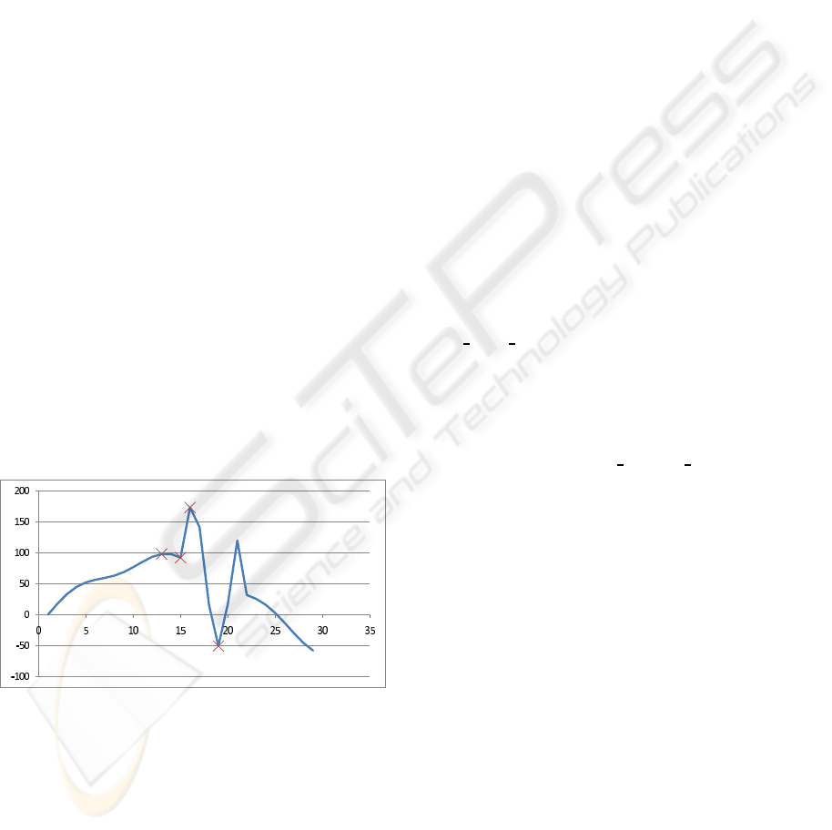
create additional extremes to ensure this condition.
The weak point of these two methods is the estimate
of additional extremes x-coordinates.
When edges of the processed signal contain time-
short components of significantly higher frequency
(in our case artifacts), the insufficiency of methods
is apparent. So, the problem surfaces distinctively
when we use artificial signals with randomly placed
artifacts.
When we calculate a new extreme with mirror
method we get a new minimum with x-coordinate:
Min
x
(0) = Max
x
(1) − (Min
x
(1) − Max
x
(1)) =
13− (15− 13) = 11
Index of a sample was used as the x-coordinate.
The new minimum is at the position of the 11
th
sam-
ple. Therefore we cannot create envelope covering all
the data.
Similar problem appears when we use the slope
based method to estimate x-coordinates of new ex-
tremes:
Max
x
(0) = Max
x
(1) − ∆t
max
(1) = Max
x
(1) −
(Max
x
(2) − Max
x
(1))
Max
x
(0) = 13− (16 − 13) = 10
Min
x
(0) = Min
x
(1) − ∆t
min
(1) = Min
x
(1) −
(Min
x
(2) − Min
x
(1))
Min
x
(0) = 15− (19 − 15) = 11
We also use the index of the sample as the x-
coordinate. Newly estimated extremes have its x-
coordinate before the beginning of the signal. So we
cannot construct the proper envelope for the sifting
process.
Figure 4: Detail of the EEsignal with artifact.
4 CONCLUSIONS
The Hilbert-Huang transform seems to be very
promising method for analysis of quasi-stationary
data series (signals). The HHT can offer very high
time-frequency resolution which makes it perfectly
suitable for our task (ERP detection when process-
ing EEG). Also, we have to keep in mind that HHT
is recently developed method and it has some issues
which have to be solved before its application.
ACKNOWLEDGEMENTS
This work was supported by Grant Agency of the
Czech Republic under the grant GA 102/07/1191.
REFERENCES
D˝atig, M. and Schlurmann, T. (2004). Performance and
limitations of the hilbert-huang transformation (hht)
with an application to irregular water waves. Ocean
engineering, 31.
Huang, N. and Attoh-Okine, N. O. (2005). The Hilbert-
Huang Transform in Engineering. CRC Press.
Huang, N. E. and et al. (1998). The empirical mode decom-
position and the hilbert spectrum for nonlinear and
non-stationary time series analysis. Proceedings of
the Royal Society of London. Series A: Mathematical,
Physical and Engineering Sciences.
Liu, R. (2002). Empirical mode decomposi-
tion: A useful technique for neuroscience?
http://techtransfer.gsfc.nasa.gov/downloads/Huang
etal98 review.pdf.
Luck, S. (2005). An Introduction to the Event-Related Po-
tential Technique. The MIT Press, Cambridge,.
Marple, L. (1999). Computing the
discrete-time ”analytic” signal via fft.
http://classes.engr.oregonstate.edu/eecs/winter2009
/ece464/AnalyticSignal Sept1999 SPTrans.pdf.
Mathworks (2010). Signal processing toolbox - hilbert.
http://www.mathworks.com/access/helpdesk/help/
toolbox/signal/index.html.
Qu, L. and Wu, F. (2008). An improved method for re-
straining the end effect in empirical mode decomposi-
tion and its applications to the fault diagnosis of large
rotating machinery. Journal of Sound and Vibration
314, Journal of Sound and Vibration:586–602.
Sanei, S. and Chambers, J. (2007). EEG Signal Processing.
John Wiley and Sons, New York,.
EMD OVERSHOOT EFECT IN ERP DETECTION ERP - Detection related Specifics of the Empirical Mode
Decomposition in EEG Analysis
241
