
COMPARISON AMONG ITERATIVE ALGORITHMS
FOR PHASE RETRIEVAL
Wooshik Kim
Sejong University, Seoul, 143-747, Republic of Korea
Keywords: Phase retrieval problem, Fourier transform, Magnitude retrieval problem, Signal reconstruction.
Abstract: Phase retrieval problem is a problem of reconstructing a signal or the phase of Fourier transform of the
signal from the magnitude of its Fourier transform. In this paper we address the problem of reconstructing
an unknown signal from the magnitude of its Fourier transform and the magnitude of Fourier transform of
another signal that is given by the addition of a known reference signal. In addition to a brief summary of
the uniqueness conditions under which a signal can be uniquely specified from the given information, we
present a simple justification that an iterative algorithm converges to the unknown original signal. And we
compare three of the iterative algorithms developed so far.
1 INTRODUCTION
The phase retrieval problem is the problem of
reconstruction of a signal from the magnitude of its
Fourier transform (or Fourier intensity). This
problem arises in a variety of different applications
including X-ray crystallography, electron
microscopy, astronomy, optics, and signal
processing (Hayes 1980, Ramachandran 1970,
Hayes 1982). This problem, however, is not easy to
solve because this problem does not have a unique
solution in general. For example, suppose we have
the magnitude of the Fourier transform of a signal. If
the signal is one-dimensional, we can make an
infinite number of different sequences which have
the same magnitude by convolving many different
all-pass sequences. Even though we restrict the
signal to be finite, we can find many other signals
which have the same Fourier transform magnitude
by the process called `zero flipping' (Hayes 1980). If
the signal is two-dimensional, even though we know
that almost all two-dimensional sequences have
irreducible z-transforms and can be uniquely defined
to within a trivial ambiguity, we cannot present a
practical and efficient algorithm to perform the
reconstruction.
To overcome the difficulties associated with the
reconstruction of a signal from its Fourier intensity,
a group of researchers have proposed many different
methods by adding additional information (Kim
1990a, Kim 2004, Fiddy 1983) or using window
functions (Nakajima 1987, Kim 1993, Kim 2008), or
using partial information such as one bit of phase
information (Van Hove 1983).
Among these, in (Kim 1990a), the authors
considered the phase retrieval using a known
additive signal. The authors presented several
conditions under which a signal is determined
uniquely from the two magnitudes of Fourier
transforms: one is the magnitude of the Fourier
transform of an unknown, desired signal and the
other is the magnitude of the Fourier transform of
another signal that is given by the addition of the
desired signal and a known ‘reference’ signal. Also,
the authors presented closed-form algorithms that
can determine the unknown, desired signal from the
given information. These closed-form algorithms,
however, may be very sensitive to noise especially
to computational noise, which may cause the
propagation of errors because they are derived from
the autocorrelations so that they are composed of
recursive equations. As results, the noise levels are
different at different locations of the solution. On the
other hand, iterative algorithms have two important
advantages over recursive algorithms. One is that, at
each stage of the iterative algorithms, we can put
various constraints such as the positivity, the finite
region of support, or the magnitude constraints. The
other is that with the control over the number of
iterations, the iterative algorithms may be terminated
at any time before the effects of noise becomes
serious.
In (Kim 1990b), the author had presented an
iterative algorithm and shown a justification that the
112
Kim W. (2010).
COMPARISON AMONG ITERATIVE ALGORITHMS FOR PHASE RETRIEVAL.
In Proceedings of the International Conference on Signal Processing and Multimedia Applications, pages 112-117
DOI: 10.5220/0002980801120117
Copyright
c
SciTePress

algorithm converges in the sense that the defined
error criterion converges to zero. Also, the paper had
presented an example that shows that the solution
signal actually converges to the unknown desired
signal. However, the paper had not given a proof
that the updated signal converges to the exact
solution signal.
In this paper we consider the same phase
retrieval problem that had been considered in (Kim
1990a). After we mention some of the uniqueness
conditions given in (Kim 1990a), we present a
corollary that may be used during the development
of the algorithm and develop an iterative algorithm.
We introduce the iterative algorithm developed in
(Kim 1990b) and present a simple justification at the
algorithm actually converges to the unknown desired
signal. Finally we present performance analysis
among the 3 iterative algorithms that can be applied
to the phase retrieval problem, i.e., Fienup algorithm
(Gerchberg-Saxton algorithm), the algorithm
developed in (Kim 1990b), and an adaptive
relaxation algorithm.
2 UNIQUENESS
In this section, we present some of the uniqueness
conditions in (Kim 1990a). Since the properties of
the one-dimensional signals are very different from
those of two- or higher dimensional signals, we first
mention the one-dimensional signals (Kim 1990a).
2.1 One-dimensional Case
To begin with, we assume that )(nx be an unknown
desired signal that is a real and discrete-time
sequence of length N. To be more specific, we
assume that
)(nx has its region of support
]1,0[ −NR , 0)0( ≠x , and 0)1( ≠−Nx . Let
)(ny be another sequence which is derived from
)(nx by the addition of a known reference sequence
)(nh , i.e.,
)()()( nhnxny +=
(1)
Now, we assume that the given information is the
two magnitudes of Fourier transforms,
|)(|
ω
j
eX ,
|)(|
ω
j
eY , and the known signal )(nh .
According to Theorem 3 in (Kim 1990a), the
unknown desired signal
)(nx can be uniquely
defined from the given information if the z-
transform of the nonlinear phase part of
)(nh does
not divide
)(zX the z-transform of )(nx . In
mathematical terms, let
)(zH be factored as
)()()( zHzAzH
lp
=
, (2)
where )()(
0
2
zHzzH
lp
n
lp
−
±= is the z-transform of a
finite length linear phase signal
)(nh
lp
.
This uniqueness condition can be put this way.
Let
)(
ˆ
nx be another signal such that its satisfies all
the conditions given to
)(nx . Then the phase of
Fourier transform of
)(
ˆ
nx is related with the phase
of the Fourier transform of
)(nx by either
)()(
ˆ
ωφωφ
X
X
=
or
)()(2)(
ˆ
ωφωφωφ
XH
X
−=
. If
)(nx is uniquely defined from the given condition
such as in Theorem 3 in (Kim 1990a), then
)(
ˆ
ω
φ
X
should satisfy
)()(2)(
ˆ
ωφωφωφ
XH
X
−≠
. This can
be summarized into the next corollary.
Corollary 1
Let
)(nx and )(ny be real, non-symmetric, finite-
length sequences such that they satisfy all the
conditions given in Theorem 3 in (Kim 1990a) such
that
)(nx can be determined uniquely from the
given conditions. Let
)(
ˆ
nx and )(
ˆ
ny be other
signals that satisfy all the conditions given to
)(nx
and
)(ny as in Theorem 3 in (Kim 1990a),
respectively. If
)(nx is uniquely defined from the
given conditions, then
)()(2)(
ˆ
ωφωφωφ
XH
X
−≠
, (3)
where
)(
ˆ
ωφ
X
, )(
ω
φ
X
, and )(
ω
φ
H
are the phases of
the Fourier transforms of
)(
ˆ
nx , )(nx , and )(nh ,
respectively.
The proof can be done easily. Let
)(
ˆ
nx and
)(
ˆ
ny be other signals that satisfy all the conditions
given in the corollary 1. Then, we have
))()(cos(|)(||)(|2
|)(||)(||)(|
222
ωφωφ
ωω
ωωω
HX
jj
jjj
eHeX
eHeXeY
++
+=
))()(cos(|)(||)(
ˆ
|2
|)(||)(
ˆ
||)(
ˆ
|
ˆ
222
ωφωφ
ωω
ωωω
H
X
jj
jjj
eHeX
eHeXeY
++
+=
Equating the two equations, we get
))()(cos())()(cos(
ˆ
ω
φ
ω
φ
ω
φ
ω
φ
H
X
HX
+=
+
If we solve this equation, then we get either
)()(
ˆ
ω
φ
ω
φ
X
X
=
or
)(2)()(
ˆ
ω
φ
ω
φ
ω
φ
HX
X
−
=
.
Since the first equation means
)()(
ˆ
nxnx = , the
satisfaction of the second equation means there
exists more than one signal that satisfies all the
conditions given, which violates the uniqueness
condition. Thus
)(
ˆ
ω
φ
X
should be
)(2)()(
ˆ
ωφωφωφ
HX
X
−≠
.
As a simple example, suppose that the given
additive reference signal
)(nh is a point sequence
such that
COMPARISON AMONG ITERATIVE ALGORITHMS FOR PHASE RETRIEVAL
113

)()(
0
nnAnh −=
δ
(4)
According to Theorem 2 in (Kim 1990a), there
exist only two sequences that satisfy the given two
magnitudes conditions. There are
)(nx and
)2(
0
nnx − (Kim 1990a). Furthermore, if we specify
the region of support of the sequences, then we can
remove this ambiguity. Since without loss of
generality we can assume that
)(nx is a finite length
sequence such that it has its region of support
]1,0[ −NR with 0)0( ≠x and 0)1( ≠−Nx . Then
the two signals
)(nx and )2(
0
nnx − will have the
same region of support only when
N is odd and
2/)1(
0
−= Nn .
2.2 Two- or Higher-dimensional Case
For the two- or higher-dimensional signals, the
uniqueness conditions are very similar to those of
the one-dimensional signals except that the
properties of two- or higher-dimensional signals are
very much different from those of one-dimensional
signals. Unlike the z-transforms of one-dimensional
signals, the z-transforms of almost all the multi-
dimensional signals are irreducible such that almost
all of the z-transforms of the two- or higher
dimensional signals are composed of only one factor
(Hayes 1982b). This means that unless the additive
reference signal
)(nh
G
is a point signal, in almost all
cases the uniqueness condition can be guaranteed.
3 ITERATIVE ALGORITHM
AND ITS CONVERGENCE
Having established conditions under which a signal
is uniquely defined in terms of the two magnitudes
of Fourier transforms, we consider an iterative
algorithm that may reconstruct the desired unknown
signal from the given information. The main frame
of the algorithm is given in (Kim 1990b). In (Kim
1990b), the author had shown that the algorithm
converges in the sense that the defined error
criterion
)(
ω
k
E converges to 0. In this section, we
first introduce the algorithm briefly and present a
simple justification that the algorithm converges to
the desired solution signal.
To develop the iterative algorithm, note from (1)
that the magnitude of the Fourier transform
)(ny is.
related to Fourier transforms of
)(nx and )(nh as
follows
)()()()(
|)(||)(||)(|
**
222
ωωωω
ωωω
jjjj
jjj
eHeXeHeX
eHeXeY
++
+=
(5)
Now we define
222
|)(||)(||)(|)(
ωωωω
jjjj
eHeXeYeK −−= (6)
Then from Eq. (5), we have
)()()()()(
**
ωωωωω
jjjjj
eHeXeHeXeK += (7)
where )(
ω
j
eK can be determined uniquely from the
given information, i.e., two Fourier intensities and
the given additive reference signal. Using the
method of successive approximations, we may then
establish the following update equation for the
iterative algorithm for finding a solution
)(
ω
j
eX
.
)]()()()(
)()[()()(
**
1
ωωωω
ωωω
ωβ
jj
k
jj
k
jj
k
j
k
eHeXeHeX
eKeXeX
−−
+=
+
(8)
Here, )(
ω
β
is a function that is used to control the
convergence of the algorithm. To see how this
algorithm works, define the error
)(
1
ω
j
k
eE
+
at the
)1(
+
k st stage of the iteration as follows
)()(
)()()()(
*
1
*
11
ωω
ωωωω
jj
k
jj
k
jj
k
eHeX
eHeXeKeE
+
++
−
−=
(9)
Using (5) in (6) it may be shown that the error at the
)1(
+
k st stage is related to the error at the k th stage
by
)()}]()(Re{21[
)()()()()()(
*
*
1
*
11
ωω
ωωωωωω
ωβ
j
k
j
jj
k
jj
k
jj
k
eEeH
eHeXeHeXeKeE
⋅−=
−−=
+++
(10)
Now, if we let )(
ω
β
be a real-valued function
of
ω
, it follows that )(
ω
j
k
eE will converge to 0
provided
1)}()(Re{0
*
<<
ω
ωβ
j
eH (11)
Therefore, if we set
0
)}](sgn[Re{)(
βωβ
ω
⋅=
j
eH (12)
where
0
β
is a positive constant such that
|})](Re{/(max{|10
0
ω
β
j
eH<< (13)
then, for each
ω
, )()(
1
ω
ω
kk
EE
<
+
will converge to
0 as
∞
→k and )()()()(
*
ωωωω
jj
k
jj
k
eHeXeHeX +
converges to
)(
ω
j
eK .
Now, we are going to show that
)(
ω
k
E converges
to 0 means that
)(
ω
j
k
eX converges to )(
ω
j
eX .
From Eq. (8), this equation can be rewritten as
)()(
)]()()()(
)()[()]()([
*
*
1
ωωβ
ωβ
ωωωω
ωωω
k
jj
k
jj
k
jj
k
j
k
E
eHeXeHeX
eKeXeX
=
−−
=−
+
(14)
SIGMAP 2010 - International Conference on Signal Processing and Multimedia Applications
114
From (14), we get
1
)(
)(
)()(
)()(
1
1
121
<=
−
−
+
+
+
ω
ω
ωω
ωω
k
k
j
k
j
k
j
k
j
k
E
E
eXeX
eXeX
(15)
Thus, as k goes to infinity, the update equation (8)
converges to some signal, say )(
ω
j
eX
∞
.
Now, we are going to see the converged signal
)(
ω
j
eX
∞
converges to the desired signal )(
ω
j
eX . If
we take a limit
∞→k to (8), we get
)]()()()(
)()[()()(
**
ωωωω
ωωω
ωβ
jjjj
jjj
eHeXeHeX
eKeXeX
∞∞
∞∞
−−
+=
(16)
or, combining (7), we get
))()(cos(|)(||)(|
))()(cos(|)(||)(|
ωφωφ
ωφωφ
ωω
ωω
hX
jj
hX
jj
eHeX
eHeX
−=
−
∞
∞
(17)
where ))(exp(|)(|)(
ωφ
ωω
∞
∞∞
=
X
jj
jeXeX .
If we solve the equation above, we get either
)()(
ω
φ
ω
φ
XX
→
∞
(18)
or
)()(2)(
ω
φ
ω
φ
ω
φ
XHX
−→
∞
. (19)
According to Corollary 1, )(nx can be uniquely
determined from the given condition, if
)()(2)(
ω
φ
ω
φ
ω
φ
XhX
−≠
∞
. This means that
)()(
ω
φ
ω
φ
XX
→
∞
and the update equation )(
ω
j
k
eX
converges to
)(
ω
j
eX , which means )()(
ˆ
nxnx → ,
in turn.
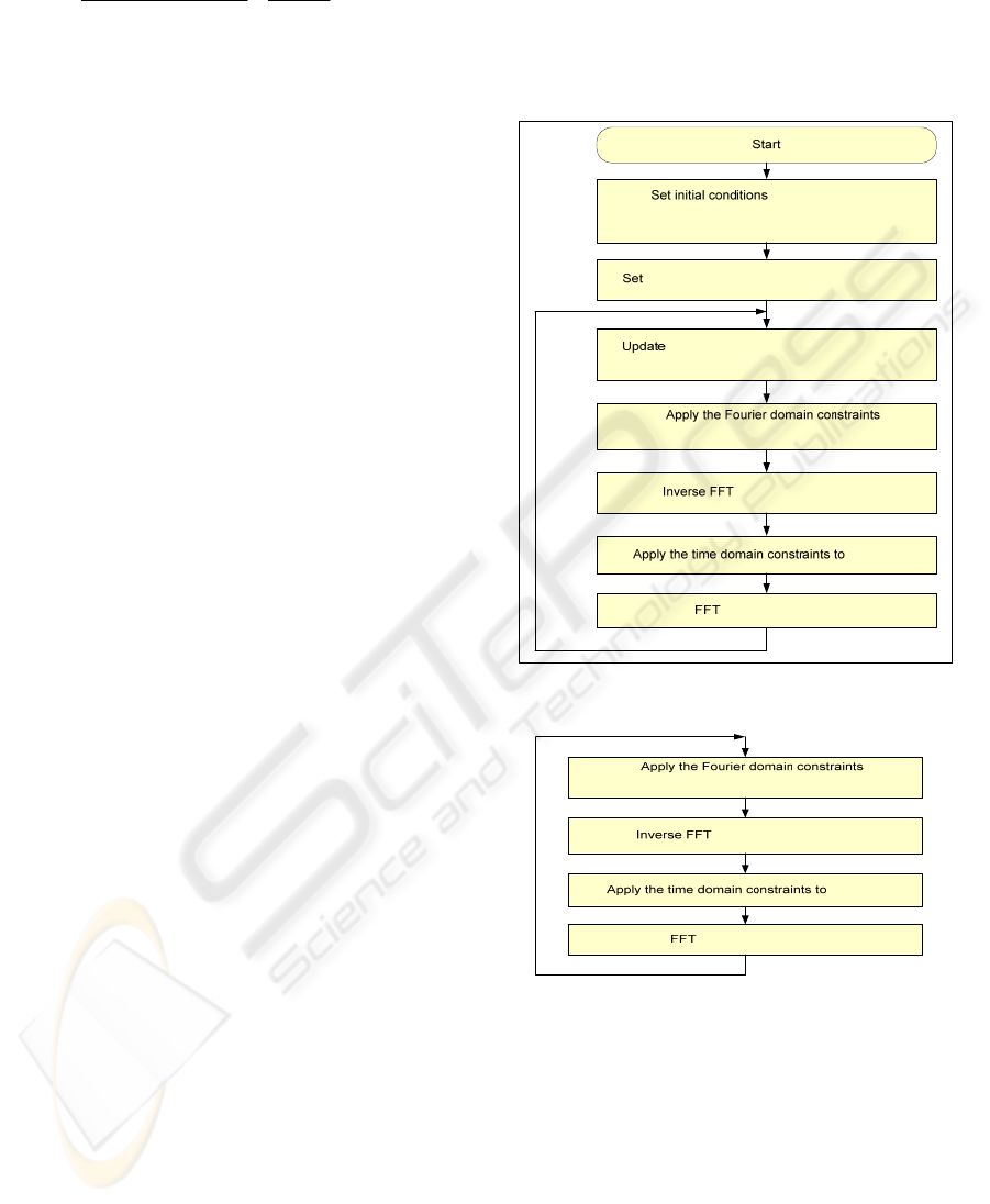
The block diagram of the developed iterative
algorithm is shown in Figure 1.
4 RECONSTRUCTION
In this section, we consider the performance
comparison of 3 iterative algorithms. One is the
described in Section 3. The second is Gerchberg-
Saxton algorithm, also known as Fienup algorithm,
which is the most basic and fundamental one to the
algorithms in phase retrieval problem area
(Gerchberg 1972). The block diagram of the GS
algorithm is given in Figure 2. This algorithm has a
very simple structure. Basically while we take
Fourier transform and inverse Fourier transform the
solution signal back and forth, we put various
constraints to the solution signal. For example, if the
solution is in time-domain, then the constraints of
finite-support, non-negativity, real signal are used. If
the solution signal is in Fourier domain, then we use
magnitude or phase constraints. One of the
characteristics of the Gerchberg-Saxton algorithm is
that if the problem satisfies the uniqueness as in the
magnitude retrieval problems, then this algorithm
has a tendency to find the exact solution (Hayes
1980). If not, as in the general phase retrieval
problem, this algorithm usually does not
converge to the solution.
222
0
|)(||)(||)(|)(
0)(
ωωωω
ω
HXYK
X
−−=
=
0
)}(sgn{Re{)(
βωωβ
⋅= H
)]()()[()()(
)()()()()(
1
**
ωωωβωω
ωωωωω
kkk
kkk
KKXX
HXHXK
−+=
+=
+
|)(||)(|
1
ω
ω
XX
k
=
+
)(
1
ω
+k
X
)(
1
nx
k +
)(
1
nx
k +
Figure 1: The block diagram of the iterative algorithm.
|)(||)(|
1
ωω
XX
k
=
+
)(
1
ω
+k
X
)(
1
nx
k +
)(
1
nx
k +
Figure 2: The block diagram of Gerchberg-Saxton
algorithm.
The final algorithm is the combination of the first
iterative algorithm and adaptive relaxation algorithm.
The adaptive relaxation algorithm is an algorithm
whose update equation is given as
)}({)()1()(
1
nxTnxnx
kkkkk
λ
λ
+
−
=
+
(20)
where )}({ nxT
k
is an constraint operator such as
time-domain or frequency-domain constraint
operator as is given in GS algorithm or the iterative
COMPARISON AMONG ITERATIVE ALGORITHMS FOR PHASE RETRIEVAL
115
algorithm in Figure 1 and
k
λ
is the relaxation
parameter (Hayes 1982a). This parameter can be
determined to minimize the error energy such that
2
]}{[
)]}{([
kk
F
kkk
F
k
xxT
xxTx
−
−
−=
∑
∑
λ
(21)
where F implies the region that the constraints are
applied to (Hayes 1982a). The block diagram of the
algorithm is given in Figure 3.
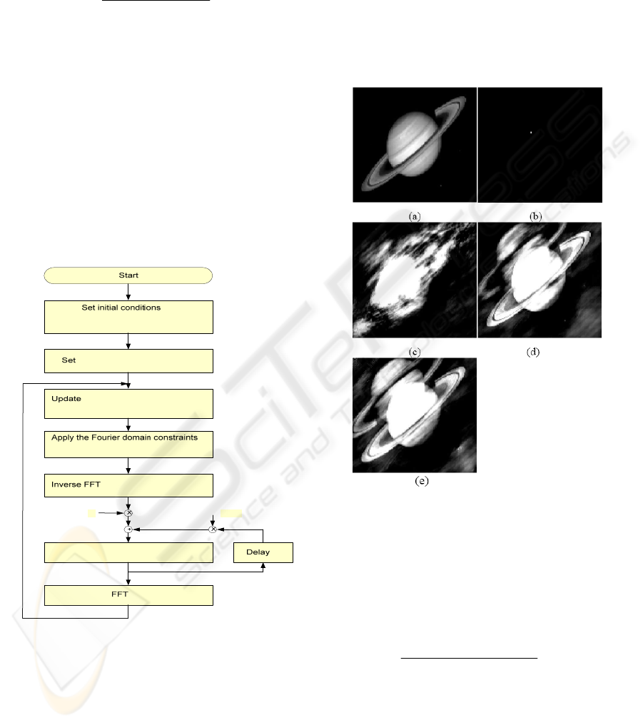
As a simulation, we present a result that shows the
performance of the algorithm. Fig. 4 (a) is the
picture of a two dimensional original signal having
128 x 128 pixels which is assumed to be unknown
and the magnitude of its Fourier transform is given.
The additive reference signal is shown (b). The
reference signal
),( nmh is assumed to be given as
⎩
⎨
⎧
×∈
=
otherwise
nm
nmh
0
]56,55[]51,50[),(255
),(
222
0
|)(||)(||)(|)(
0)(
ωωωω
ω
HXYK
X
−−=
=
0
)}(sgn{Re{)(
βωωβ
⋅= H
)]()()[()()(
)()()()()(
1
**
ωωωβωω
ωωωωω
kkk
kkk
KKXX
HXHXK
−+=
+=
+
|)(||)(|
1
ωω
XX
k
=
+
)(
1
ω
+k
X
}{)()1()(
1 kkkkk
xTnxnx
λλ
+−=
+
)(
1
nx
k +
k
λ
)1(
k
λ
−
Figure 3: The block diagram of the combination of the
iterative algorithm in Figure 2 and adaptive relaxation.
which is a 2x2 square box but may look like a
blurred point signal.
Then the another magnitude of the signal
),(),(),( nmhnmxnmy
+
=
is assumed to be given. Since the maximum value
of
),(
21
ωω
jj
eeH is 255*2*2 = 1020, the
convergence constant
0
β
should be greater than
zero and less than 1/(255*2*2)=
04
1089039.9
−
× and
in this case we picked
04
0
1089039.9
−
×=
β
. Figure
(c), (d), and (e) show the images that are
reconstructed by Gerchberg-Saxton algorithm ,
Iterative algorithm, and Adaptive relaxation
algorithm, respectively, after 20 iterations. In these
pictures, we can see that while the result from
Gerchberg-Saxton algorithm does not converge to
the desired signal, the signals reconstructed by the
other two algorithms looks similar to the desired
signal and thus converge to the desired signal.
Figure 4: The original signal and the reconstructed signals
after 20 iterations; (a). the original signal, (b) the additive
reference signal, (c) the reconstructed signal using the GS
algorithm, (d) using the iterative algorithm, and (e) the
algorithm with adaptive relaxation.
Figure 5 shows the comparison between the
performances of the 3 algorithms. The mean squared
error here is defined as
[
]
N
M
nmxnmx
MSE
ro
×
−
=
∑
2
),(),(
where
NM
×
is the number of pixels in ),( nmx .
As we can see in this picture, the Gerchberg-Saxton
algorithm does neither diverge nor converge. On the
`other hand, the iterative algorithm converges as
iteration goes on constantly. On the other hand, in
the beginning part of the simulation, the algorithm
with adaptive relaxation converges quickly.
However, the algorithm saturated and does not
SIGMAP 2010 - International Conference on Signal Processing and Multimedia Applications
116
converge any more. Obviously, the optimal
algorithm is in the beginning part of the iteration, the
algorithm needs to follow the adaptive relaxation
property and later to follow the iterative algorithm.
Figure 5: Comparison of the convergence properties
between the GS algorithm, the iterative algorithm, and
algorithm with adaptive relaxation.
Finally, in Figure 6, we presented the reconstructed
algorithm after 100 iterations using the iterative
algorithm. As we had given the justification, the
algorithm converges and the reconstructed signal
actually converges to the desired signal.
Figure 6: An example that shows the convergence
property of the iterative algorithm. (a) The original image
and (b) the reconstructed image after 100 iterations using
the iterative algorithm.
5 CONCLUSIONS
In this paper we considered the problem of
iteratively reconstructing a one-dimensional or a
two-dimensional signal from a pair of Fourier
intensities: the intensity of the signal along with the
intensity of another signal that is related by the
addition of a known reference signal. After we
present the uniqueness of the solution briefly, we
presented a simple proof that the iterative algorithm
converges the desired original signal, which is
assumed to be unknown. The algorithm combined
with the iterative algorithm and the adaptive
relaxation algorithm converges fast in the beginning
part and however goes saturated fastly also. Future
work may be the evaluating the robustness of the
algorithms to noise in the measured intensities and
methods of improving the convergence properties of
the constrained iterative algorithm.
ACKNOWLEDGEMENTS
This work was supported by the Korea Research
Foundation Grant funded by the Korean
Government (2009-0072495).
REFERENCES
Hayes, M. H., Lim, J. S., and Oppenheim, A. V., 1980,
Signal reconstruction from phase or magnitude, IEEE
Tr. ASSP., 28, 672-680.
Ramachandran G.N., and Srinivasan, R. (1970), Fourier
methods in crystallography, Wiley-Interscience, NY.
Hayes, M. H., 1982a, The reconstruction of a
multidimensional sequence from the phase or
magnitude of its Fourier transform, IEEE Tr. ASSP,
30, 140-154.
Kim, W. and Hayes, M. H., 1990a, Phase retrieval using
two Fourier transform intensities”, J. Opt. So. Am. A,
7, 441-449.
Kim, W., 2004, Two-dimensional phase retrieval using
enforced minimum-phase signals, J. Kor. Phy. Soc.,
44, 287-292.
Fiddy, M. A., Brames, B. J., and Dainty, J. C., 1983,
Enforcing irreducibility for phase retrieval in two
dimensions, Opt. Lett. 8, 96-98.
Nakajima, N., 1987, Phase retrieval from two intensity
measurements using the Fourier series expansion, J.
Opt. Soc. Am. A, 4, 154-158.
Kim W. and Hayes, M. H., 1993, Phase retrieval using a
window function, IEEE Tr. SP., 41, 1409 - 1412.
Kim W., 2008, Phase retrieval by enforcing the off-axis
holographic condition, J. Kor. Phy. Soc., 52, 264-268.
Van Hove, P.L., Hayes, M. H., Lim, J.S., and Oppenheim,
A.V., 1983, Signal reconstruction from signed Fourier
transform magnitude, IEEE Tr. ASSP, 31, 1286-1293.
Kim, W. and Hayes M.H., 1990b, Iterative phase retrieval
using two Fourier transform intensities, Proceedings,
ICASSP. Albuquerque, NM. April 3-6. D:1563-1566.
Hayes, M. H. and McClellan, J.H., 1982b, Reducible
polynomial in more than one variable, IEEE Proc., 70,
197-198.
Gerchberg, R.W. and Saxton, W.O., 1972, A practical
algorithm for the determination of the phase from
image and diffraction plane pictures, Optik 35, 237-
246.
COMPARISON AMONG ITERATIVE ALGORITHMS FOR PHASE RETRIEVAL
117
